
数据结构与算法
1.时间复杂度与排序
时间复杂度:只取系数最高项,且忽略最高项系数剩下的。
$an_2+bn+c$的时间复杂度可以用$O(n_2)$表示
排序方式
选择排序
先在前n个数中选取最小值排到第一位,再在后面n-1个数中选取最小数放到这n-1个数的第一位。
#include<iostream>
using namespace std;
void Select_Sort(int arr*,int n)
{
    for(int i = 0;i < n;i++){
        int min = i;
        for(int j = i;j < n;j++){
            if(arr[min] > arr[j]){
                min = j;
            }
        }
        if(min != i){
            swap(arr[i],arr[min]);
        }
    }

}
package class01;
import java.util.Arrays;
public class Code01_SelectionSort{
public static void selectionSort(int[] arr){
if(arr == null||arr.length < 2){
return 0;
}
for(int i = 0,i < arr.length - 1; i++){
int minIndex = i;
for(int j = i+1,j<arr.length,j++){
minIndex = arr[j] < arr[minIndex] ? j : minIndex;//此时出用到了三目运算符[布尔表达式 ? 取真时取值 : 取假时取值]
}
swap(arr, i, minIndex);
}
}
public static void swap(int[] arr,int i,int j){
int tmp = arr[i];
arr[i] = arr[j];
arr[j] = tmp;
}
}冒泡排序
先对从0到n-1项进行相邻两项的大小排序,再对从0到n-2项进行相邻大小排序,以此类推,最终排序完成。
public class Bubble_Sort{
    public static void bubbleSort(int[] arr){
        if(arr == null || arr.length == 1) return 0;
        for(int i = 0;i < arr.length - 1;i++){
            boolean isSorted = ture;
            for(int j = 0;j < arr.length - 1 - i;j++){
                if(arr[j] > arr[j + 1]){
                    int temp = arr[j];
                    arr[j] = arr[j + 1];
                    arr[j + 1] = temp;
                    isSorted = false;
                }
            }
        if(isSorted) return;
        System.out.print("第"+(i+1)+"趟:");
        print(arr);
        }
    }
}
package class01;
import java.util.Arrays;
public class Code02_BubbleSort{
public static void bubbleSort(int[] arr){
if(arr = null||arr.length < 2){
return;
}
for(int n = arr.length - 1,n > 0,n--){
for(int i = 0,i < e,i++){
if(arr[i] > arr[i+1]){
swap(arr,i,i + 1);
}
}
}
}
public static void swap(int[] arr,int i,int j){
arr[i]=arr[i]^arr[j];
arr[j]=arr[i]^arr[j];
arr[i]=arr[i]^arr[j];
}
}^ 异或运算(不同为1,相同为0)
相关性质:
0 ^ N = N

N ^ N = N

满足交换律和结合率

一群数异或先后顺序不影响结果

注意:亦或运算中的两个数字位置不能指向同一片内存区域
算法题
//数组内某个数出现了奇数次,其他数字出现了偶数次,求该出现了基数次的数
public static void print0ddTimesNum1(int[] arr){
    int eor = 0;
    for(int cur : arr){
        eor ^= cur;
    }
    System.out.println(eor);
}
数组内某两个数出现了奇数次,其他数字出现偶数次,求这两个数
public static void print0ddTimesNum2(int[] arr){
    int eor = 0;
    for(int i = 1,i < arr.length;i++){
        eor ^arr[i];
    }
    int rightone = eor & (~eor + 1);
    int onlyOne = 0;    //onlyOne就是eor'
    for (int cur : arr){
        if((cur & rightOne) == 0){
            onlyOne ^= cur;
        }
    }
    System.out.println(onlyOne + " " +(eor ^ onlyOne));
}
两个奇数次数,先异或运算获得第一个奇数次数,再 eor ^ eor ' 即可得到第二个奇数次数
插入排序
先看 0\~0上是否有序,再看 0\~1上是否有序,有序则不变,无序则排序以此类推到最后 0\~n。该算法与所给数据的不同复杂度也不同。
时间复杂度为O($N^2$),额外空间复杂度为O(1)。
public class Code03_InsertionSort{
    public static void insortionSort(int[] arr){
        if(arr == null||arr.length < 2){
            return;
        }
        for(int i = 1;i < arr.length;i++){
            for(int j = i - 1;j >= 0 && arr[j] > arr[j+1];j--){
                swap(arr,j,j+1);
            }
        }
    }
    public static void swap(int[] arr,int i,int j){
        arr[i] = arr[i] ^ arr[j];
        arr[j] = arr[i] ^ arr[j];
        arr[i] = arr[i] ^ arr[j];
    }
}
二分法查找
二分法要在已经排好序的数组中进行查找,先和中间数比较再与下一段的中间数比较,时间复杂度为$log_2N$。
二分法还可以找大于等于某数最左侧的数字和小于等于某数最右侧的位置都可以。
算法题
在一个数组arr中,arr无序,且任意两个相邻的数不相等,定义局部最小,只求一个局部最小,问是否存在一个算法复杂度可以小于O(n)。
解法:
若 0\~1中与N-2\~N-1中趋势不同则再数组中必定存在局部最小,二分法求中间两个数的大小关系,和哪边相同就往反方向继续二分。

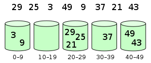
希尔排序
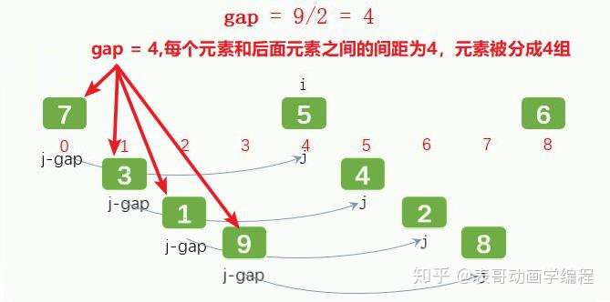
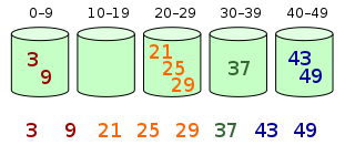
希尔排序,通过增量(gap)将元素两两分组,对每组使用直接插入排序算法排序;增量(gap)逐渐减少,当增量(gap)减至1时,整个数据恰被分成一组,最后进行一次插入排序,整个数组就有序了。

第一次:gap = 9/2 = 4,每个元素和后面的元素之间间隔4,元素被分成4组。其中元素7, 5, 6分成一组,元素3,4分成一组,元素1, 2分成一组,元素9,8分成一组,效果如下图:
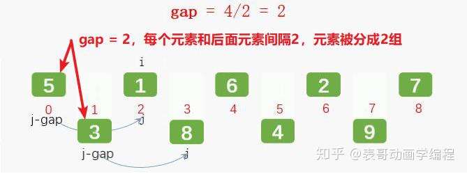
第二次:gap = 4/2 = 2,每个元素和后面的元素之间间隔2,元素被分成2组。
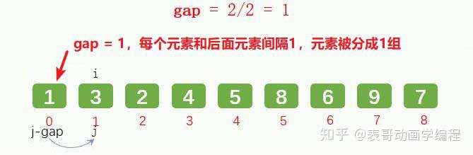
第三次:gap = 2/2 = 1,每个元素和后面的元素之间间隔1,元素被分成1组。
public class ShellSortTest2 {
    public static void main(String[] args) {
        int[] arr = new int[] {7, 3, 1, 9, 5, 4, 2, 8, 6};
        shellSort(arr);
    }

    public static void shellSort(int[] arr) {
        // 增量gap,通过gap来划分出不同的子序列,gap不断减少,划分的子序列更多
        for (int gap = arr.length / 2; gap > 0; gap /= 2) { // 循环得到不同的gap,gap = 4, 2, 1
            System.out.println("gap: " + gap);

            for (int i = gap; i < arr.length; i++) { // 每组使用插入排序
                for (int j = i; j-gap >= 0; j -= gap) {
                    if (arr[j-gap] > arr[j]) {
                        swap(arr, j-gap, j);
                        System.out.print("\t交换: " + arr[j-gap] + "和" + arr[j]);
                        System.out.println(Arrays.toString(arr));
                    }
                }
            }
        }
    }

    public static void swap(int[] arr, int start, int end) {
        int temp = arr[start];
        arr[start] = arr[end];
        arr[end] = temp;
    }
}
执行效果:
gap: 4
    交换: 5和7[5, 3, 1, 9, 7, 4, 2, 8, 6]
    交换: 8和9[5, 3, 1, 8, 7, 4, 2, 9, 6]
    交换: 6和7[5, 3, 1, 8, 6, 4, 2, 9, 7]
gap: 2
    交换: 1和5[1, 3, 5, 8, 6, 4, 2, 9, 7]
    交换: 4和8[1, 3, 5, 4, 6, 8, 2, 9, 7]
    交换: 2和6[1, 3, 5, 4, 2, 8, 6, 9, 7]
    交换: 2和5[1, 3, 2, 4, 5, 8, 6, 9, 7]
gap: 1
    交换: 2和3[1, 2, 3, 4, 5, 8, 6, 9, 7]
    交换: 6和8[1, 2, 3, 4, 5, 6, 8, 9, 7]
    交换: 7和9[1, 2, 3, 4, 5, 6, 8, 7, 9]
    交换: 7和8[1, 2, 3, 4, 5, 6, 7, 8, 9]
总结
希尔排序,是直接插入排序算法的一种更高效的改进版本。通过增量(gap)将元素进行分组,对每组使用直接插入排序算法排序;增量(gap)逐渐减少,当增量(gap)减至1时,整个数据恰被分成一组,最后进行一次插入排序。
对数器
1、生成随机样本产生器。
2、将两个方法同时输入数据,比较两个方法的方法。
public static void comparator(int[] arr){
    Arrays.sort(arr);
}
java生成随机数的函数
//自己打的
public static int[] generateRandomArray(int maxSize,int maxValue){
    //(int)(Math.random() * N) ——>[0 ~ N-1]所有的整数,等概率返回一个
    int[] arr = new int[(int)((maxSize + 1) * Math.random())];
    for (int i = 0;i < arr.length;i++){
        arr[i] = (int)((maxValue + 1) * Math.random()) - (int)(maxValue * Math.random());
    }
    return arr;
}
//网上的
//随机数组的生成
//Math.random() [0,1) double
//Math.random() *A ->[0,A) double A->int
public static int []generateRandomArray(int maxSize,int maxValue)
{
    int []arr=new int[(int)(maxSize+1)*Math.random())];
    for(int i=0;i<arr.length;i++)
    {
        arr[i]=(int)((maxValue+1)*Math.random())-(int)(maxValue*Math.random)
    }
    return arr;

}
//复制 返回数组
public static int[] copyArray(int[] arr)
{
    if(arr==null)
    {
        return null;
    }
    int []res=new int[arr.length];
    for(int i=0;i<arr.length;i++)
    {
        res[i]=arr[i];
    }
    return res;
}
测试器案例
//for test
static void main()
{
     int testTime=2000;//测试次数
     int maxSize=100;//数组大小
     int maxValue=100;//数组值大小
     boolean succeed=true;//初始值 不成功
     for(int i=0;i<testTime;i++)
     {
       int []arr1=generateRandomArray(maxSize,maxValue);//产生随机数组
       int []arr2=copyArray(arr1);                      //拷贝生成新数组
       selectionSort(arr1);                             //被测黑盒函数
       comparator(arr2);                                //绝对正确函数
       if(!isEqual(arr1,arr2))                          //对比结果
        {
           succeed=false;                           //只要有一次失败就打印
           printArray(arr1);
           printArray(arr2);
           break;
         }
      }
}
2.认识O(NlogN)的排序
取中点的方法:
$$
mid = \frac{L+R}{2}
$$
但是这种方法不一定准确,如果在数组中R足够的大,可能会造成溢出,从而mid取负数。
故采用以下方法:
$$
mid = L + \frac{R-L}{2}
$$
同时为了提高运算效率引入位运算符>>
$$
mid = L + ((R-L)>>1)
$$
位运算符 >> or <<
将左边的数转换成二进制数,再根据符号方向向左或向右移动一定位数,这个位数指的是符号右边的值。
递归法求最大值
public class Code08_GetMax{
    public static int getMax(int[] arr){
        return process(arr, 0, arr.length - 1);
    }
    public static int process(int[] arr, int L, int R){
        if(L == R){
            return arr[L];
        }
        int mid = L + ((R - L) >> 1);
        int leftMax = process(arr, L, mid);
        int rightMax = process(arr, mid + 1, R);
        return Math.max(leftMax, rightMax);
    }
}
master公式——解递归程序复杂度的方法
$$
master\;公式:T(N) = a \times T(\frac{N}{b}) +O(N^d)\
关于\,master\,公式有以下结论:\
若\;log_ba<d,则该递归复杂度为\;O(N^d)\
若\;log_ba>d,则该递归复杂度为\;O(N^{log_ba})\
若\;log_ba=d,则该递归复杂度为\;O(N^d \times logN)
$$


归并排序
左边排好序,右边排好序让整体有序,时间复杂度由 master 公式求出,为$O(N\times logN)$,额外空间复杂度为$O(N)$。
在额外一个空间内,左右依次相同序号的数字比较,谁小先拷贝谁到新空间内。最终再拷贝回原数组。

//归并排序代码实现
import java.util.Arrays;
public class Code01_MergeSort{
    public static void mergeSort(int[] arr){
        if(arr = null || arr.length < 2){
            return;
        }
        process(arr, 0, arr.length - 1);
    }
    public static void process(int[] arr, int L, int R){
        if(L == R){
            return;
        }
        int mid = L + ((R - L) >> 1);
        process(arr, L, mid);
        process(arr, mid + 1, R);
        merge(arr, L, mid, R);
    }
    public static void merge(int[] arr, int L, int M, int R){
        int[] help = new int[R - L + 1];
        int i =0;
        int p1 = L;
        int p2 = M + 1;
        while(p1 <= M && p2 <= R){
            help[i++] = arr[p1] <=arr[p2] ? arr[p1] :arr[p2];
        }
        while(p1 <= M){
            help[i++] = arr[p1++];
        }
        while(p2 <= R){
            help[i++] = arr[p2++];
        }
        for (i = 0; i < help.length; i++){
            arr[L + i] = help[i++];
        }
    }
}

之前的排序在比较以后丢弃了大量的比较数据。

笨方法是暴力求解,较好的算法是运用归并排序进行计算。如图:

//实现代码
class test
{   public static int smallSum(int[] arr) {
    if (arr == null || arr.length < 2) {
        return 0;
    }
    return mergeSort(arr, 0, arr.length - 1);
}

 public static int mergeSort(int[] arr, int l, int r) {
     if (l == r) {
         return 0;
     }
     int mid = l + ((r - l) >> 1);
     return mergeSort(arr, l, mid) + mergeSort(arr, mid + 1, r) + merge(arr, l, mid, r);
 }

 public static int merge(int[] arr, int l, int m, int r) {
     int[] help = new int[r - l + 1];
     int i = 0;
     int p1 = l;
     int p2 = m + 1;
     int res = 0;
     while (p1 <= m && p2 <= r) {
         res += arr[p1] < arr[p2] ? (r - p2 + 1) * arr[p1] : 0;
         help[i++] = arr[p1] < arr[p2] ? arr[p1++] : arr[p2++];
     }
     while (p1 <= m) {
         help[i++] = arr[p1++];
     }
     while (p2 <= r) {
         help[i++] = arr[p2++];
     }
     for (i = 0; i < help.length; i++) {
         arr[l + i] = help[i];
     }
     return res;
 }
 public static void main (String[] args) throws java.lang.Exception
 {
     int[] arr = { 1,2,3};
     System.out.println(smallSum(arr));
 }
}
问题一:分两步:
[i] <= num , [i] 和<=边界的下一个数字交换,小于区域右移,i++;
[i] > num , i++
问题一衍生:增加等于区域

快速排列
选择最后一个数,将数组划分成两部分,再分别对两部分的最后一个数重复进行上述步骤。快速排序的时间复杂度最差为O(N),空间复杂度最差为O(N),按照概率相关知识,得出快速排序的时间复杂度为O(NlogN),空间复杂度是O(logN)。

快速排序使用分治法(Divide and conquer)策略来把一个序列(list)分为两个子序列(sub-lists)。
① 从数列中挑出一个元素,称为 “基准”(pivot),
② 重新排序数列,所有元素比基准值小的摆放在基准前面,所有元素比基准值大的摆在基准的后面(相同的数可以到任一边)。在这个分区退出之后,该基准就处于数列的   中间位置。这个称为分区(partition)操作。
③ 递归地(recursive)把小于基准值元素的子数列和大于基准值元素的子数列排序。
递归到最底部时,数列的大小是零或一,也就是已经排序好了。这个算法一定会结束,因为在每次的迭代(iteration)中,它至少会把一个元素摆到它最后的位置去。
划分值取的好的话,数据结构时间复杂度可以达到 NlogN。

将划分值看成等概率好坏,再对不同情况下的master公式求数学期望,可得数学时间复杂度为O(NlogN)。
//快速排序相关代码
public static void quickSort(int[] arr){
    if(arr == null || arr.length<2){
        return;
    }
    quickSort(arr,0,arr.length-1);
}
public static void quickSort(int[] arr,int l,int r){
    if(l < r){
        swap(arr, l+(int)(Math.random()*(r-l+1)),r);//随机抽取数值
        int[] p = partition(arr,l,r);//将等于x部分筛出,存放至数组之中。
        quickSort(arr,l,p[0]-1);//小于部分快速排序
        quickSort(arr,p[1]+2,r);//大于部分快速排序
    }
}
public static int[] partition(int[] arr,int l,int r){
    int less = l-1;
    int more = r;
    //将r当作该数值,将r-1个数值进行比较,最后再将more和r进行转换。
    while(l<more){
        if(arr[l]<arr[r]){
            swap(arr,++less,l++);
        }else if(arr[l]>arr[r]){
            swap(arr,--more,l);
        }else{
            l++
        }
    }
    swap(arr,more,r);
    return new int[] { less+1,more};
}
public static void swap(int[] arr,int i,int j){
    int tmp = arr[i];
    arr[i] = arr[j];
    arr[j] = tmp;
}
堆
在逻辑上是完全二叉树

堆排序

让用户输入的数字变成大根堆。
heapinsert
(1).顺序插入。
(2).将数字和父位置的根节点比较,比根节点大则跟换位置,不大则顺序排列。
(3).和更高的根节点比较,更换。
如果要删除大根堆的根节点怎么处理?
heapify
将最后一个数字放到第一个位置,heapsize - 1;
将该数字与左子树,右子树根节点比较,交换;
重复上个步骤。
//heapinsert相关代码
public static void heapInsert(int [] arr, int index){
while(arr[index] > arr[(index - 1)/2]){
swap(arr, index, (index - 1) /2);
index = (index - 1) /2;
}
}
public static void heapify(int[] arr, int index, int heapSize){
int left = index * 2 + 1;
while (left < heapSize){
int largest = left + 1 < heapSize && arr[left > 1] > arr[left] ? left + 1 : left;
//上述式子理解:先对(left + 1 < heapSize)(arr[left > 1] > arr[left])分别进行判断,再进行逻辑与&&运算,正确取左,不正确取右,最后赋值。
largest = arr[largest] > arr[index] ? largest : index;
if(largest == index){
break;
}
swap(arr, largest, index);
index = largest;
left = index * 2 + 1;
}
}
public static void swap(intp[] arr, int i, int j){
int temp = arr[i];
arr[i] = arr[j];
arr[j] = temp;
}//堆排序code
public static void Code02_HeapSort{
public static void heapSort(int [] arr){
if(arr = null || arr.length < 2){
return;
}
// for(int i = 0, i < arr.length, i++){
// heapInsert(arr, i);
// }
for(int i = arr.length - 1;i >= 0;i--){
heapify(arr, i, arr.length);
}//该方法比上面的注释内容略快,但不影响整体的复杂度。
int heapSize = arr.length;
swap(arr, 0, --heapSize);
while(heapSize > 0){
heapify(arr, 0, heapSize);
swap(arr, 0, --heapSize);
}
}
}堆排序的时间复杂度为O(NlogN),额外空间复杂度为O(1)。
如果直接给n个数的数组,从右至左,从下往上heapify。


其复杂度为O(logk)。
优先队列
#include<iostream>
#include<queue>
using namespace std;
int main()
{
    priority_queue<int>heap;
    heap.push(10);
    heap.push(8);
    heap.push(9);
    heap.push(12);
    heap.push(3);

    while(heap.size()>0)
    {
        cout<<heap.top()<<" ";
        heap.pop();
    }
    return 0;
}
import java.util.PriorityQueue;
public class04_SortArrayDistanceLessK{
    public void sortedArrayDistanceLessK(int [] arr, int k){
        //默认小根堆,系统优先排序。
        PriorityQueue<Integer> heap = new PriorityQueue<>();
        int index = 0;
        for(; index <= Math.min(arr.length,k);index++){
            heap.add(arr[index]);
        }
        int i = 0;
        for(;index <= arr.length; index++){
            heap.add(arr[index]);
            arr[i] = heap.poll();
        }
        while(!heap.isEmpty()){
            arr[i++] = heap.poll();
        }
    }
    public static void main(String [] args){
        PriorityQueue<Integer> heap = new PriorityQueue<>();
        heap.add(8);
        heap.add(4);
        heap.add(4);
        heap.add(9);
        heap.add(10);
        heap.add(3);
        while(!heap.isEmpty()){
            System.out.println(heap.poll());
        }//>>>3 4 4 8 9 10
    }
}
比较器


3.桶排序以及排序内容大总结
计数排序
计数排序(Counting sort)是一种稳定的线性时间排序算法。
1. 基本思想
计数排序使用一个额外的数组C,其中第i个元素是待排序数组A中值等于i的元素的个数。
计数排序的核心在于将输入的数据值转化为键存储在额外开辟的数组空间中。作为一种线性时间复杂度的排序,计数排序要求输入的数据必须是有确定范围的整数。
用来计数的数组C的长度取决于待排序数组中数据的范围(等于待排序数组的最大值与最小值的差加上1),然后进行分配、收集处理:
① 分配。扫描一遍原始数组,以当前值-minValue作为下标,将该下标的计数器增1。
② 收集。扫描一遍计数器数组,按顺序把值收集起来。
2. 实现逻辑
① 找出待排序的数组中最大和最小的元素
② 统计数组中每个值为i的元素出现的次数,存入数组C的第i项
③ 对所有的计数累加(从C中的第一个元素开始,每一项和前一项相加)
④ 反向填充目标数组:将每个元素i放在新数组的第C(i)项,每放一个元素就将C(i)减去1
3. 动图演示
计数排序演示
举个例子,假设有无序数列nums=[2, 1, 3, 1, 5], 首先扫描一遍获取最小值和最大值,maxValue=5, minValue=1,于是开一个长度为5的计数器数组counter
(1) 分配
统计每个元素出现的频率,得到counter=[2, 1, 1, 0, 1],例如counter[0]表示值0+minValue=1出现了2次。
(2) 收集
counter[0]=2表示1出现了两次,那就向原始数组写入两个1,counter[1]=1表示2出现了1次,那就向原始数组写入一个2,依次类推,最终原始数组变为[1,1,2,3,5],排序好了。
4. 复杂度分析
平均时间复杂度:O(n + k)
最佳时间复杂度:O(n + k)
最差时间复杂度:O(n + k)
空间复杂度:O(n + k)
当输入的元素是n 个0到k之间的整数时,它的运行时间是 O(n + k)。。在实际工作中,当k=O(n)时,我们一般会采用计数排序,这时的运行时间为O(n)。
计数排序需要两个额外的数组用来对元素进行计数和保存排序的输出结果,所以空间复杂度为O(k+n)。
计数排序的一个重要性质是它是稳定的:具有相同值的元素在输出数组中的相对次序与它们在输入数组中的相对次序是相同的。也就是说,对两个相同的数来说,在输入数组中先出现的数,在输出数组中也位于前面。
计数排序的稳定性很重要的一个原因是:计数排序经常会被用于基数排序算法的一个子过程。我们将在后面文章中介绍,为了使基数排序能够正确运行,计数排序必须是稳定的。
5. 代码实现
C版本:
// 计数排序(C)
#include <stdio.h>
#include <stdlib.h>
#include <time.h>
void print_arr(int *arr, int n) {
    int i;
    printf("%d", arr[0]);
    for (i = 1; i < n; i++)
        printf(" %d", arr[i]);
    printf("\n");
}
void counting_sort(int *ini_arr, int *sorted_arr, int n) {
    int *count_arr = (int *) malloc(sizeof(int) * 100);
    int i, j, k;
    for (k = 0; k < 100; k++)
        count_arr[k] = 0;
    for (i = 0; i < n; i++)
        count_arr[ini_arr[i]]++;
    for (k = 1; k < 100; k++)
        count_arr[k] += count_arr[k - 1];
    for (j = n; j > 0; j--)
        sorted_arr[--count_arr[ini_arr[j - 1]]] = ini_arr[j - 1];
    free(count_arr);
}
int main(int argc, char **argv) {
    int n = 10;
    int i;
    int *arr = (int *) malloc(sizeof(int) * n);
    int *sorted_arr = (int *) malloc(sizeof(int) * n);
    srand(time(0));
    for (i = 0; i < n; i++)
        arr[i] = rand() % 100;
    printf("ini_array: ");
    print_arr(arr, n);
    counting_sort(arr, sorted_arr, n);
    printf("sorted_array: ");
    print_arr(sorted_arr, n);
    free(arr);
    free(sorted_arr);
    return 0;
}
Java版本:
// 计数排序(Java)
public class CountingSort {
    public static void main(String[] argv) {
        int[] A = CountingSort.countingSort(new int[]{16, 4, 10, 14, 7, 9, 3, 2, 8, 1});
        Utils.print(A);
    }
    public static int[] countingSort(int[] A) {
        int[] B = new int[A.length];
        // 假设A中的数据a'有,0<=a' && a' < k并且k=100
        int k = 100;
        countingSort(A, B, k);
        return B;
    }
    private static void countingSort(int[] A, int[] B, int k) {
        int[] C = new int[k];
        // 计数
        for (int j = 0; j < A.length; j++) {
            int a = A[j];
            C[a] += 1;
        }
        Utils.print(C);
        // 求计数和
        for (int i = 1; i < k; i++) {
            C[i] = C[i] + C[i - 1];
        }
        Utils.print(C);
        // 整理
        for (int j = A.length - 1; j >= 0; j--) {
            int a = A[j];
            B[C[a] - 1] = a;
            C[a] -= 1;
        }
    }
}
6. 优化改进
场景分析:举个极端的例子:如果排序的数组有200W个元素,但是这200W个数的值都在1000000-1000100,也就说有100个数,总共重复了200W次,现在要排序,怎么办?
这种情况排序,计数排序应该是首选。但是这时候n的值为200W,如果按原来的算法,k的值10001000,但是此时c中真正用到的地方只有100个,这样对空间造成了极大的浪费。
改进思路:针对c数组的大小,优化计数排序
改进代码:
// 计数排序优化(Java)
// 针对c数组的大小,优化计数排序
public class CountSort{
    public static void main(String []args){
        //排序的数组
        int a[] = {100, 93, 97, 92, 96, 99, 92, 89, 93, 97, 90, 94, 92, 95};
        int b[] = countSort(a);
        for(int i : b){
            System.out.print(i + "  ");
        }
        System.out.println();
    }
    public static int[] countSort(int []a){
        int b[] = new int[a.length];
        int max = a[0], min = a[0];
        for(int i : a){
            if(i > max){
                max = i;
            }
            if(i < min){
                min = i;
            }
        }
        //这里k的大小是要排序的数组中,元素大小的极值差+1
        int k = max - min + 1;
        int c[] = new int[k];
        for(int i = 0; i < a.length; ++i){
            c[a[i]-min] += 1;//优化过的地方,减小了数组c的大小
        }
        for(int i = 1; i < c.length; ++i){
            c[i] = c[i] + c[i-1];
        }
        for(int i = a.length-1; i >= 0; --i){
            b[--c[a[i]-min]] = a[i];//按存取的方式取出c的元素
        }
        return b;
    }
}
三、总结
计数算法只能使用在已知序列中的元素在0-k之间,且要求排序的复杂度在线性效率上。 Â 计数排序和基数排序很类似,都是非比较型排序算法。但是,它们的核心思想是不同的,基数排序主要是按照进制位对整数进行依次排序,而计数排序主要侧重于对有限范围内对象的统计。基数排序可以采用计数排序来实现。
桶排序
桶排序是计数排序的升级版。它利用了函数的映射关系,高效与否的关键就在于这个映射函数的确定。为了使桶排序更加高效,我们需要做到这两点:
- 在额外空间充足的情况下,尽量增大桶的数量
- 使用的映射函数能够将输入的 N 个数据均匀的分配到 K 个桶中
同时,对于桶中元素的排序,选择何种比较排序算法对于性能的影响至关重要。
1. 什么时候最快
当输入的数据可以均匀的分配到每一个桶中。
2. 什么时候最慢
当输入的数据被分配到了同一个桶中。
3. 示意图
元素分布在桶中:
然后,元素在每个桶中排序:
public class BucketSort implements IArraySort {

    private static final InsertSort insertSort = new InsertSort();

    @Override
    public int[] sort(int[] sourceArray) throws Exception {
        // 对 arr 进行拷贝,不改变参数内容
        int[] arr = Arrays.copyOf(sourceArray, sourceArray.length);

        return bucketSort(arr, 5);
    }

    private int[] bucketSort(int[] arr, int bucketSize) throws Exception {
        if (arr.length == 0) {
            return arr;
        }

        int minValue = arr[0];
        int maxValue = arr[0];
        for (int value : arr) {
            if (value < minValue) {
                minValue = value;
            } else if (value > maxValue) {
                maxValue = value;
            }
        }

        int bucketCount = (int) Math.floor((maxValue - minValue) / bucketSize) + 1;
        int[][] buckets = new int[bucketCount][0];

        // 利用映射函数将数据分配到各个桶中
        for (int i = 0; i < arr.length; i++) {
            int index = (int) Math.floor((arr[i] - minValue) / bucketSize);
            buckets[index] = arrAppend(buckets[index], arr[i]);
        }

        int arrIndex = 0;
        for (int[] bucket : buckets) {
            if (bucket.length <= 0) {
                continue;
            }
            // 对每个桶进行排序,这里使用了插入排序
            bucket = insertSort.sort(bucket);
            for (int value : bucket) {
                arr[arrIndex++] = value;
            }
        }

        return arr;
    }

    /**
     * 自动扩容,并保存数据
     *
     * @param arr
     * @param value
     */
    private int[] arrAppend(int[] arr, int value) {
        arr = Arrays.copyOf(arr, arr.length + 1);
        arr[arr.length - 1] = value;
        return arr;
    }

}
基数排序
以十进制三位数的数组为例,准备10个桶,分别对应 0~9的基数位,首先根据个位数决定进哪个桶,对个位数进行排序;再以十位数决定进哪个桶,对十位数进行排序;最后因为排序优先级是从十位到个位的,就可以得到整体有序的数组。


处理以后变为:

//arr[L...R]排序 digit是最大的数字有多少个十进制位,
//也就是最大值的数 位数
public static radixSort(int[] arr,int L,int R,int digit)
{
    final int radix=10;
    int i=0,j=0;
    //有多少个数准备多少个辅助空间
    int[] bucket=new int[R-L+1];
    //有多少位就操作几次
    for(int d=1;d<=digit;d++)
    {

        int[] count=new int[radix];

        for(i=L;i<=R;i++)
        {
            //得到倒数第d位上的数字是几
            j=getDigit(arr[i],d);
            count[j]++;
        }
        //创建count‘数组,count[0]上的数字不变
        for(i=1;i<radix;i++)
            count[i]=count[i]+count[i-1];

        //从右向左遍历arr数组
        for(i=R;i>=L;i--)
        {
            j=getDigit(arr[i],d);
            bucket[arr[j]-1]=arr[i];
            count[j]--;
        }

        //把某一位有序的数组copy回原数组
        for(i=L,j=0;i<=R;i++,j++)
        {
            arr[i]=bucket[j];
        }

    }
}

//返回x这个数在倒数第d位上的数是几
public static int getDigit(int x,int d)
{
    return ( ( x/ ( (int)Math.pow(10,d-1) ) ) %10 );
}

//返回最大值的位数
public static int maxbits(int[] arr){
    int max=Integer.MIN_VALUE;
    for(int i=0;i<arr.length;i++)
    {
        max=Math.max(max,arr[i]);
    }
    int res=0;
    while(max!=0){
        res++;
        max/=10;
    }
    return res;
}

public static void main()
{
    int[] arr={022,021,032,001,100}
    if(arr==null||arr.length<2){
        return;
    }
    radixSort(arr,0,arr.length-1,maxbits(arr));
}
排序总结


4.链表
链表基础知识
链表的概念
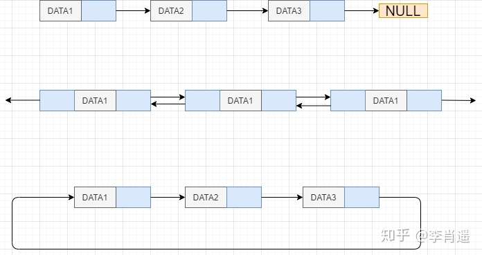
链表的基本思维是,利用结构体的设置,额外开辟出一份内存空间去作指针,它总是指向下一个结点,一个个结点通过NEXT指针相互串联,就形成了链表。

链表的结构是多式多样的,当时通常用的也就是两种:

- 无头单向非循环列表:结构简单,一般不会单独用来存放数据。实际中更多是作为其他数据结构的子结构,比如说哈希桶等等。
- 带头双向循环链表:结构最复杂,一般单独存储数据。实际中经常使用的链表数据结构,都是带头双向循环链表。这个结构虽然复杂,但是使用代码实现后会发现这个结构会带来很多优势,实现反而简单了。
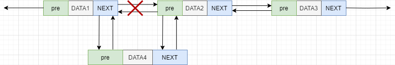
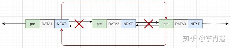
插入删除操作只需要修改指针所指向的区域就可以了,不需要进行大量的数据移动操作。如下图:

链表包含单链表、双链表、循环链表,如下图:
单链表
//单链表的节点定义
typedef struct Node {
    int data;       //数据类型,你可以把int型的data换成任意数据类型,包括结构体struct等复合类型
    struct Node *next;          //单链表的指针域
} Node,*LinkedList;
//Node表示结点的类型,LinkedList表示指向Node结点类型的指针类型
//链表初始化
//创建一个单链表的前置节点并向后逐步添加节点,一般指的是申请结点的空间,同时对一个结点赋空值(NULL)
LinkedList listinit(){
    Node *L;
    L=(Node*)malloc(sizeof(Node));      //开辟空间
    if(L==NULL){                     //判断是否开辟空间失败,这一步很有必要
        printf("申请空间失败");
        //exit(0);                  //开辟空间失败可以考虑直接结束程序
    }
    L->next=NULL;       //指针指向空
}
创建单列表有两种方式,==头插入法与尾插入法==
利用指针指向下一个结点元素的方式进行逐个创建,使用头插入法最终得到的结果是逆序的。如图所示:

//头插法建立单链表
LinkedList LinkedListCreatH() {
    Node *L;
    L = (Node *)malloc(sizeof(Node));   //申请头结点空间
    L->next = NULL;                      //初始化一个空链表

    int x;                         //x为链表数据域中的数据
    while(scanf("%d",&x) != EOF) {
        Node *p;
        p = (Node *)malloc(sizeof(Node));   //申请新的结点
        p->data = x;                     //结点数据域赋值
        p->next = L->next;     //将结点插入到表头L-->|2|-->|1|-->NULL
        L->next = p;
    }
    return L;
}
如图所示为尾插入法的创建过程:

//尾插法建立单链表
LinkedList LinkedListCreatT() {
    Node *L;
    L = (Node *)malloc(sizeof(Node));   //申请头结点空间
    L->next = NULL;                  //初始化一个空链表
    Node *r;
    r = L;                          //r始终指向终端结点,开始时指向头结点
    int x;                         //x为链表数据域中的数据
    while(scanf("%d",&x) != EOF) {
        Node *p;
        p = (Node *)malloc(sizeof(Node));   //申请新的结点
        p->data = x;                     //结点数据域赋值
        r->next = p;            //将结点插入到表头L-->|1|-->|2|-->NULL
        r = p;
    }
    r->next = NULL;
    return L;
}
//遍历单链表
//遍历输出单链表
void printList(LinkedList L){
Node *p=L->next;
int i=0;
while(p){
printf("第%d个元素的值为:%d\n",++i,p->data);
p=p->next;
}
}
//链表内容的修改,在链表中修改值为x的元素变为为k。
LinkedList LinkedListReplace(LinkedList L,int x,int k) {
Node *p=L->next;
int i=0;
while(p){
if(p->data==x){
p->data=k;
}
p=p->next;
}
return L;
}单链表的插入与删除


//单链表的插入与删除
LinkedList LinkedListInsert(LinkedList L,int i,int x) {
    Node *pre;                      //pre为前驱结点
    pre = L;
    int tempi = 0;
    for (tempi = 1; tempi < i; tempi++) {
        pre = pre->next;                 //查找第i个位置的前驱结点
    }
    Node *p;                                //插入的结点为p
    p = (Node *)malloc(sizeof(Node));
    p->data = x;
    p->next = pre->next;
    pre->next = p;

    return L;
}

LinkedList LinkedListDelete(LinkedList L,int x) {
    Node *p,*pre;                   //pre为前驱结点,p为查找的结点。
    p = L->next;

    while(p->data != x) {              //查找值为x的元素
        pre = p;
        p = p->next;
    }
    pre->next = p->next;          //删除操作,将其前驱next指向其后继。
    free(p);

    return L;
}
双链表

双向链表创建的过程可以分为:创建头结点->创建一个新的结点->将头结点和新结点相互链接->再度创建新结点
typedef struct line{
    int data;           //data
    struct line *pre;   //pre node
    struct line *next;  //next node
}line,*a;
//分别表示该结点的前驱(pre),后继(next),以及当前数据(data)
//创建双链表
line* initLine(line * head){
    int number,pos=1,input_data;
    //三个变量分别代表结点数量,当前位置,输入的数据
    printf("请输入创建结点的大小\n");
    scanf("%d",&number);
    if(number<1){return NULL;} //输入非法直接结束
    //////头结点创建///////
    head=(line*)malloc(sizeof(line));
    head->pre=NULL;
    head->next=NULL;
    printf("输入第%d个数据\n",pos++);
    scanf("%d",&input_data);
    head->data=input_data;

    line * list=head;
    while (pos<=number) {
        line * body=(line*)malloc(sizeof(line));
        body->pre=NULL;
        body->next=NULL;
        printf("输入第%d个数据\n",pos++);
        scanf("%d",&input_data);
        body->data=input_data;

        list->next=body;
        body->pre=list;
        list=list->next;
    }
    return head;
}
双向链表的遍历、插入与删除:
//遍历双链表,同时打印元素数据
void printLine(line *head){
    line *list = head;
    int pos=1;
    while(list){
        printf("第%d个数据是:%d\n",pos++,list->data);
        list=list->next;
    }
}
//插入数据
line * insertLine(line * head,int data,int add){
    //三个参数分别为:进行此操作的双链表,插入的数据,插入的位置
    //新建数据域为data的结点
    line * temp=(line*)malloc(sizeof(line));
    temp->data=data;
    temp->pre=NULL;
    temp->next=NULL;
    //插入到链表头,要特殊考虑
    if (add==1) {
        temp->next=head;
        head->pre=temp;
        head=temp;
    }else{
        line * body=head;
        //找到要插入位置的前一个结点
        for (int i=1; i<add-1; i++) {
            body=body->next;
        }
        //判断条件为真,说明插入位置为链表尾
        if (body->next==NULL) {
            body->next=temp;
            temp->pre=body;
        }else{
            body->next->pre=temp;
            temp->next=body->next;
            body->next=temp;
            temp->pre=body;
        }
    }
    return head;
}
//删除元素
line * deleteLine(line * head,int data){
    //输入的参数分别为进行此操作的双链表,需要删除的数据
    line * list=head;
    //遍历链表
    while (list) {
        //判断是否与此元素相等
        //删除该点方法为将该结点前一结点的next指向该节点后一结点
        //同时将该结点的后一结点的pre指向该节点的前一结点
        if (list->data==data) {
            list->pre->next=list->next;
            list->next->pre=list->pre;
            free(list);
            printf("--删除成功--\n");
            return head;
        }
        list=list->next;
    }
    printf("Error:没有找到该元素,没有产生删除\n");
    return head;
}
两单链表相交问题
题目
- 给定两个可能是环也可能无环的单链表,头节点head1和head2.。请实现一个函数,如果两个链表相交,请返回相交的第一个节点,如果不相交,返回null。
要求
- 如果两个链表长度之和为N,时间复杂度请达到O(N),额外空间复杂度请达到O(1)。
分析
本题目可以拆分为:
问题1.如何判断单链表有环还是无环,有环返回第一个入环节点,无环返回null。

第一种方法
可以利用哈希表(hashSet):遍历每一个节点,想要把每个结点都存放到哈希表中;但是哈希表中已经存过的节点就存不进去了(第一个不能存入哈希表的节点就是第一个入环的节点)。
注:需要一个哈希表,空间复杂度O(n)不满足。
第二种方法
设定两个指针:一个快指针(走两步),一个慢指针(走一步);当快指针和慢指针相遇的时候,快指针回到头结点的位置,和慢指针一起以一步的步幅走,相遇的节点就是第一个入环节点。
public static Node getLoopNode(Node head) {
    if (head == null || head.next == null || head.next.next == null) {
        return null;
    }
    Node n1 = head.next; // n1 -> slow
    Node n2 = head.next.next; // n2 -> fast
    while (n1 != n2) {
        if (n2.next == null || n2.next.next == null) {
            return null;
        }
        n2 = n2.next.next;
        n1 = n1.next;
    }
    n2 = head; // n2 -> walk again from head
    while (n1 != n2) {
        n1 = n1.next;
        n2 = n2.next;
    }
    return n1;
}
问题2.两个无环链表怎么找到第一个相交的节点

第一种方法
利用哈希表:
遍历第一个链表,把所有的节点都存入到哈希表中(因为是无环链表,所以一定可以存进去)(哈希表中存放的节点的内存地址,和节点的值没有关系);遍历第二个链表的节点,每遍历一个查看哈希表中是否已经有了这个节点,哈希表中第一个存不进去的节点就是第一个相交节点。
哈希表空间复杂度是O(n),不满足题目要求。
第二种方法
1.先确定两个链表的长度差
2.两个链表在移动的过程中,如果相交了(根据链表的特殊性,只有一个next指针,只能连接一个下一个结点,所以第一个公共结点之后,只知道链表的结尾都是相同的)(变量中存放的是内存地址,和数据无关),那么末尾的内存地址一定是相同的
3.如果最后的相等,那么说明是有相交的节点的,但是不一定是最后一个。
4.让长的节点从头开始,先走距离差个距离;短的从头开始走,相等的就是他们相交的节点
public static Node noLoop(Node head1, Node head2) {
    if (head1 == null || head2 == null) {
        return null;
    }
    Node cur1 = head1;
    Node cur2 = head2;
    int n = 0;
    while (cur1.next != null) {
        n++;
        cur1 = cur1.next;
    }
    while (cur2.next != null) {
        n--;
        cur2 = cur2.next;
    }
    if (cur1 != cur2) {
        return null;
    }
    cur1 = n > 0 ? head1 : head2;
    cur2 = cur1 == head1 ? head2 : head1;
    n = Math.abs(n);
    while (n != 0) {
        n--;
        cur1 = cur1.next;
    }
    while (cur1 != cur2) {
        cur1 = cur1.next;
        cur2 = cur2.next;
    }
    return cur1;
}
问题三:如何判断两个有环链表是否相交,相交则返回第一个相交节点,不相交则返回null。
考虑问题三的时候,我们已经得到了两个链表各自的第一个入环节点,假设链表 1 的第一个入环节点记为loop1,链表2 的第一个入环节点记为loop2。以下是解决问题三的过程。
1.如果loop1==loop2,那么两个链表的拓扑结构如图

这种情况下,我们只要考虑链表1 从头开始到loop1 这一段与链表2 从头开始到loop2 这一段,在那里第一次相交即可,而不用考虑进环该怎么处理,这就与问题二类似,只不过问题二是把null 作为一个链表的终点,而这里是把loop1(loop2)作为链表的终点。但是判断的主要过程是相同的。
2.如果loop1!=loop2,两个链表不相交的拓扑结构如图2-9 所示。两个链表相交的拓扑结构如图2-10 所示。

如何分辨是这两种拓扑结构的哪一种呢?进入步骤3。
3.让链表1 从loop1 出发,因为loop1 和之后的所有节点都在环上,所以 将来一定能回到 loop1。
如果回到loop1 之前 并没有遇到loop2,说明两个链表的拓扑结构如图2-9 所示,也就是 不相交,直接返回 null;
如果回到loop1 之前 遇到了loop2,说明两个链表的拓扑结构如图2-10所示,也就是 相交。因为 loop1 和 loop2 都在两条链表上,只不过loop1 是离链表1 较近的节点,loop2 是离链表2 较近的节点。所以,此时返回loop1 或loop2 都可以。
问题三的具体实现参看如下代码中的 bothLoop 方法。
public static Node bothLoop(Node head1, Node loop1, Node head2, Node loop2) {
    Node cur1 = null;
    Node cur2 = null;
    if (loop1 == loop2) {
        cur1 = head1;
        cur2 = head2;
        int n = 0;
        while (cur1 != loop1) {
            n++;
            cur1 = cur1.next;
        }
        while (cur2 != loop2) {
            n--;
            cur2 = cur2.next;
        }
        cur1 = n > 0 ? head1 : head2;
        cur2 = cur1 == head1 ? head2 : head1;
        n = Math.abs(n);
        while (n != 0) {
            n--;
            cur1 = cur1.next;
        }
        while (cur1 != cur2) {
            cur1 = cur1.next;
            cur2 = cur2.next;
        }
        return cur1;
    } else {
        cur1 = loop1.next;
        while (cur1 != loop1) {
            if (cur1 == loop2) {
                return loop1;
            }
            cur1 = cur1.next;
        }
        return null;
    }
}
哈希表
UnOrderMap UnSortedMap UnOrderSet UnSortedSet-->C++
Map:Key -> Value
Set:Key


反转单向链表和双向链表
//反转单向链表
public static Node reverseOne(Node head){
    if(head == Null||head.next == Null){
        return head;
    }
    Node new_head = Null;
    while(head != Null){
        Node tmp = head.next;
        head.next = new_head;
        new_head = head;
        head = tmp;
    }
    return new_head;
}
//反转双向链表
public static DoubleNode reverse(DoubleNode head) {
if (head == null || head.next == null) {
return head;
}
DoubleNode pre = null;
DoubleNode next = null;
while (head != null) {
next = head.next;
head.next = pre;
head.last = next;
pre = head;
head = next;
}
return pre;
}打印两个有序列表的公共部分
上下进行比较,值小的部分指针后移再比较,知道其中一个数组越界。
public static void printCommonPart(Node head1 , Node head2){
    System.out.println("common part:");
    while(head1!=null && head2!=null){
        if(head1.value<head2.value){
            head1=head1.next;
        }else if(head1.value >head2.value){
            head2=head2.next;
        }else {
            System.out.println(head1.value + "");
            head1 = head1.next;
            head2 = head2.next;
        }
    }
    System.out.println();
}
判断单链表是否是回文结构
- 利用栈先进后出的特性,将链表中的元素放进栈内,再将栈内元素提出做比较,若全部相等则是回文结构。
- 将栈后半边的元素放入栈与前一半元素作比较,若全部相等则证明是回文结构(实现方式:快慢指针)。
- 最优方法,右侧链表反向,依次与左边作比较,全部相等则是回文结构。
package class04;

import java.util.Stack;

public class Code04_IsPalindromeList {

    public static class Node {
        public int value;
        public Node next;

        public Node(int data) {
            this.value = data;
        }
    }
    // need n extra space
    public static boolean isPalindrome1(Node head) {
        Stack<Node> stack = new Stack<Node>();//新建栈
        Node cur = head;//遍历链表用的,另外一个Node head
        while (cur != null) {//压栈
            stack.push(cur);
            cur = cur.next;
        }
        while (head != null) {
            if (head.value != stack.pop().value) {
                return false;
            }
            head = head.next;
        }
        return true;
    }
将单链表转化成左边小,中间相等,左边大的形式。
//链表结构如下:
public static class Node {
    public Node next;
    public int value;

    public Node(int data) {
        value = data;
    }
}
基础解法
思路
- 按链表顺序,用数组装每一个节点
- 用荷兰国旗算法对数组排序,其实就是快拍的partition过程
- 将数组还原为链表
public static Node listPartition1(Node head, int pivot) {
    if (head == null) {
        return head;
    }
    Node cur = head;
    int i = 0;
    while (cur != null) {
        i++;
        cur = cur.next;
    }
    Node[] nodeArr = new Node[i];
    cur = head;
    // 把链表的值复制到数组中
    for(i = 0; i < nodeArr.length; i++) {
        nodeArr[i] = cur;
        cur = cur.next;
    }
    // 对数据进行“荷兰国旗”分组
    arrPartition(nodeArr, pivot);
    // 重新把链表连接
    for(i = 1; i < nodeArr.length; i++) {
        nodeArr[i - 1].next = nodeArr[i];
    }
    nodeArr[i - 1].next = null;
    return nodeArr[0];
}
/// 荷兰国旗算法
public static void arrPartition(Node[] nodeArr, int pivot) {
    int more = nodeArr.length;
    int less = -1;
    int i = 0;
    while(i != more) {
        if (nodeArr[i].value < pivot) {
            less++;
            swap(nodeArr, less, i);
            i++;
        }else if(nodeArr[i].value > pivot) {
            more--;
            swap(nodeArr, i, more);
        }else {
            i++;
        }
    }
}
进阶解法
思路
- 使用6个指针建立小于,等于,大于pivot的链表区域
- 每一次遍历都更新对应区域的头尾节点
- 全部遍历节点完毕后,将连接小于的尾->等于的头->等于的尾->大于的头
public static Node listPartition2(Node head, int pivot) {
    // 小于pivot的链表头尾节点
    Node lessSt = null;
    Node lessEnd = null;
    // 等于pivot的链表头尾节点
    Node eqSt = null;
    Node eqEnd = null;
    // 大于pivot的链表头尾节点
    Node moreSt = null;
    Node moreEnd = null;
    // 用于保存next指针
    Node next = null;
    // 遍历链表
    while(head != null) {
        next = head.next;
        // 为了不污染小于,等于,大于的指针next,这里清空
        head.next = null;
        if(head.value < pivot) {
            if(lessSt == null) {
                lessSt = head;
                lessEnd = head;
            }else {
                lessEnd.next = head;
                lessEnd = head;
            }
        }else if(head.value == pivot) {
            if(eqSt == null) {
                eqSt = head;
                eqEnd = head;
            }else {
                eqEnd.next = head;
                eqEnd = head;
            }
        }else {
            if(moreSt == null) {
                moreSt = head;
                moreEnd = head;
            }else {
                moreEnd.next = head;
                moreEnd = head;
            }
        }
        head = next;
    }
    // 小于和等于区域相连
    if(lessEnd != null) {
        lessEnd.next = eqSt;
        // 判断equal的结尾指针是否为空
        eqEnd = eqEnd == null ? lessEnd : eqEnd;
    }
    // 最后等于,大于区域相连
    if (eqEnd != null) {
        eqEnd.next = moreSt;
    }
    if (lessSt != null) {
        return lessSt;
    }
    if (eqSt != null) {
        return eqSt;
    }
    if (moreSt != null) {
        return moreSt;
    }
    return null;
}
复制含有随即指针节点的链表
普通解法
首先介绍普通解法,普通解法可以做到时间复杂度为O(N),额外空间复杂度为O(N),需要使用到哈希表(HashMap)结构。具体过程如下:
-
从左到右遍历链表,对每个节点都复制生成相应的副本节点,然后将对应关系放入哈希表map 中。例如,链表1->2->3->null,遍历1、2、3 时依次生成1′、2′、3′,最后将对应关系放入map 中。

步骤1 完成后,原链表没有任何变化,每一个副本节点的next 和rand 指针都指向null。
-
再从左到右遍历链表,此时就可以设置每一个副本节点的next 和rand 指针。
例如:原链表1->2->3->null,假设1 的rand 指针指向3,2 的rand 指针指向null,3 的rand指针指向1。遍历到节点1 时,可以从map 中得到节点1 的副本节点1′,节点1 的next 指向节点2,所以从map 中得到节点2 的副本节点2′,然后令1′.next=2′,副本节点1′的next 指针就设置好了。同时节点1 的rand 指向节点3,所以从map 中得到节点3 的副本节点3′,然后令1′.rand=3′,副本节点1′的rand 指针也设置好了。以这种方式可以设置每一个副本节点的next与rand 指针。
-
将1′节点作为结果返回即可。
哈希表增删改查的操作时间复杂度都是O(1),普通方法一共只遍历链表两遍,所以普通解法的时间复杂度为O(N),因为使用了哈希表来保存原节点与副本节点的对应关系,所以额外空间复杂度为O(N)。
进阶解法
进阶解法不使用哈希表来保存对应关系,而只用有限的几个变量完成所有的功能。具体过程如下:
-
从左到右遍历链表,对每个节点cur 都复制生成相应的副本节点copy,然后把copy 放在cur 和下一个要遍历节点的中间。
例如:原链表1->2->3->null,在步骤1 中完成后,原链表变成1->1′->2->2′->3->3′->null。
-
再从左到右遍历链表,在遍历时设置每一个副本节点的rand 指针。还是举例来说明调整过程。
例如:此时链表为1->1′->2->2′->3->3′->null,假设1 的rand 指针指向3,2 的rand 指针指向null,3 的rand 指针指向1。遍历到节点1 时,节点1 的下一个节点1.next 就是其副本节点1′。1 的rand 指针指向3,所以1′的rand 指针应该指向3′。如何找到3′呢?因为每个节点的副本节点都在自己的后一个,所以此时通过3.next 就可以找到3′,令1′.next=3′即可。以这种方式可以设置每一个副本节点的rand 指针。
-
步骤2 完成后,节点1,2,3,……之间的rand 关系没有任何变化,节点1′,2′,3′……之间的rand 关系也被正确设置了,此时所有的节点与副本节点串在一起,将其分离出来即可。例如:此时链表为1->1′->2->2′->3->3′->null,分离成1->2->3->null 和1′->2′->3′->null 即可,并且在这一步中,每个节点的rand 指针不用做任何调整,在步骤2 中都已经设置好。
-
将1′节点作为结果返回即可。

import java.util.HashMap;
public class Code_13_CopyListWithRandom {
    public static class Node {
        public int value;
        public Node next;
        public Node rand;

        public Node(int data) {
            this.value = data;
        }
    }
    //方法一:采用hashMap
    public static Node copyListWithRand1(Node head) {
        HashMap<Node, Node> map = new HashMap<Node, Node>();
        Node cur = head;
        while (cur != null) {
            map.put(cur, new Node(cur.value));
            cur = cur.next;
        }
        cur = head;
        while (cur != null) {
            map.get(cur).next = map.get(cur.next);
            map.get(cur).rand = map.get(cur.rand);
            cur = cur.next;
        }
        return map.get(head);
    }
    //方法二:i 和 i’一组
    public static Node copyListWithRand2(Node head) {
        if (head == null) {
            return null;
        }
        Node cur = head;
        Node next = null;
        // copy node and link to every node
        while (cur != null) {
            next = cur.next;
            cur.next = new Node(cur.value);
            cur.next.next = next;
            cur = next;
        }
        cur = head;
        Node curCopy = null;
        // set copy node rand
        while (cur != null) {
            next = cur.next.next;
            curCopy = cur.next;
            curCopy.rand = cur.rand != null ? cur.rand.next : null;
            cur = next;
        }
        Node res = head.next;
        cur = head;
        // split
        while (cur != null) {
            next = cur.next.next;
            curCopy = cur.next;
            cur.next = next;
            curCopy.next = next != null ? next.next : null;
            cur = next;
        }
        return res;
    }
}
5.二叉树
二叉树节点结构
class Node<V>{
    V value;
    Node left;
    Node right;
}
- 用递归和非递归两种方式实现二叉树的先序,中序,后序遍历
- 直观打印一颗二叉树
- 如何完成二叉树的宽度寻优遍历
递归遍历

public static void f(Node head){
    if(head == null){
    return;
    }
    f(head.left);
    f(head.right);
}
先序、中序、后序遍历

先序遍历:对于二叉树的每一个子树都是,先打应头,再打印左孩子,再打印右孩子
思路:现将头放入一个栈中,开始遍历,遍历内容:每次从栈中弹出栈顶元素,打印栈顶元素,判断是否有右孩子,将栈顶元素右孩子压入栈中,判断是否有左孩子,再将栈顶元素的左孩子压进栈中
中序遍历
思路:先将头节点的左边界压入栈中,开始遍历,遍历内容:每次从栈中弹出栈顶元素,打印栈顶元素,判断是否有右孩子,将栈顶元素右孩子压入栈中,再将左边界都压入栈中
后序遍历
思路:现将头放入一个栈1中,开始遍历,遍历内容:每次从栈1中弹出栈顶元素,将元素放入栈2中(只有这里和前序遍历不同),判断是否有右孩子,将栈1顶元素右孩子压入栈1中,判断是否有左孩子,再将栈1顶元素的左孩子压进栈1中最后将栈2的元素一次pop出来打印
public static class Node {
    public int value;
    public Node left;
    public Node right;

    public Node(int data) {
        this.value = data;
    }
}
public static void preOrderRecur(Node head) { //先序
    if (head == null) {
        return;
    }
    System.out.print(head.value + " ");  //唯一的不同就是打印过程的位置
    preOrderRecur(head.left);
    preOrderRecur(head.right);
}
public static void inOrderRecur(Node head) {  //中序
    if (head == null) {
        return;
    }
    inOrderRecur(head.left);
    System.out.print(head.value + " ");
    inOrderRecur(head.right);
}
public static void posOrderRecur(Node head) {  //后序
    if (head == null) {
        return;
    }
    posOrderRecur(head.left);
    posOrderRecur(head.right);
    System.out.print(head.value + " ");
}
直观打印一颗二叉树
package com.gxu.dawnlab_algorithm4;
public class PrintBinaryTree {
    public static class Node{
        public int data;
        public Node left;
        public Node right;

        public Node(int data){
            this.data = data;
        }
    }

    public static void printTree(Node head){
        System.out.println("Binary Tree:");
        printInOrder(head, 0, "H", 17);
        System.out.println();
    }

    public static void printInOrder(Node head,int height,String to,int len){    //height是树高,从0层开始
        if(head == null){
            return;
        }
        printInOrder(head.right,height+1,"v",len);
        String val = to + head.data + to;
        int lenM = val.length();
        int lenL = (len - lenM) / 2;
        int lenR = len - lenM - lenL;
        val = getSpace(lenL) + val + getSpace(lenR);
        System.out.println(getSpace(height * len) + val);   //height * len空格是为了显示不同层效果
        printInOrder(head.left,height+1,"^",len);

    }

    public static String getSpace(int num){
        String space = " ";
        StringBuffer buf = new StringBuffer();
        for (int i = 0; i < num; i++) {
            buf.append(space);
        }
        return buf.toString();
    }

    public static void main(String[] args) {
        Node head = new Node(1);
        head = new Node(1);
        head.left = new Node(2);
        head.right = new Node(3);
        head.left.left = new Node(4);
        head.right.left = new Node(5);
        head.right.right = new Node(6);
        head.left.left.right = new Node(7);
        printTree(head);

    }
}
public static void printTree(Node head) {
System.out.println("Binary Tree:");
printInOrder(head, 0, "H", 17);
System.out.println();
}
public static void printInOrder(Node head, int height, String to, int len) {
if (head == null) {
return;
}
printInOrder(head.right, height + 1, "v", len);
String val = to + head.value + to;
int lenM = val.length();
int lenL = (len - lenM) / 2;
int lenR = len - lenM - lenL;
val = getSpace(lenL) + val + getSpace(lenR);
System.out.println(getSpace(height * len) + val);
printInOrder(head.left, height + 1, "^", len);
}
public static String getSpace(int num) {
String space = " ";
StringBuffer buf = new StringBuffer("");
for (int i = 0; i < num; i++) {
buf.append(space);
}
return buf.toString();
}二叉树的宽度优先遍历
方法一:hash表+队列
public static void w(Node head){
    if(head == null){
        return;
    }
    Queue<Node> queue = new LinkedList<>();
    queue.add(head);
    HashMap<Node, Integer> levelMap = new HashMap<>();
    levelMap.put(head, 1);
    int curLevel = 1;
    int curLevelNodes = 0;
    int max = Integer.MIN_VALUE;
    while(!queue.isEmpty()){
        Node cur = queue.poll();
        int curNodeLevel = levelMap.get(cur);
        if(curNodeLevel == curLevel){
            curLevelNodes++;
        }else{
            max = Math.max(max, curLevelNodes);
            curLevel++;
            curLevelNodes = 1;
        }
        if(cur.left != null){
            levelMap.put(cur.left,curNodeLevel + 1);
            queue.add(cur.left);
        }
        if(cur.right != null){
            levelMap.put(cur.right, curNodeLevel + 1);
            queue.add(cur.right);
        }
    }
    return max;
}
方法二:队列

二叉树的相关概念及其实现判断
- 如何判断二叉树是否是搜索二叉树
- 如何判断二叉树是否是完全二叉树
- 如和判断二叉树是否是满二叉树
- 如何判断二叉树是否是平衡二叉树
搜索二叉树的判断
搜索二叉树左右节点都比根节点大
//思路:中序遍历,从小到大就是
package class07;
public class Code05_IsBinarySearchTree {
    public static class TreeNode {
        public int val;
        public TreeNode left;
        public TreeNode right;
        TreeNode(int val) {
            this.val = val;
        }
    }
    public static class Info {
        public boolean isBST;
        public int max;
        public int min;
        public Info(boolean is, int ma, int mi) {
            isBST = is;
            max = ma;
            min = mi;
        }
    }
//  public static Info process(TreeNode x) {
//      if (x == null) {
//          return null;
//      }
//      Info leftInfo = process(x.left);
//      Info rightInfo = process(x.right);
//      int max = x.val;
//      int min = x.val;
//      if (leftInfo != null) {
//          max = Math.max(leftInfo.max, max);
//          min = Math.min(leftInfo.min, min);
//      }
//      if (rightInfo != null) {
//          max = Math.max(rightInfo.max, max);
//          min = Math.min(rightInfo.min, min);
//      }
//      boolean isBST = true;
//      if (leftInfo != null && !leftInfo.isBST) {
//          isBST = false;
//      }
//      if (rightInfo != null && !rightInfo.isBST) {
//          isBST = false;
//      }
//      boolean leftMaxLessX = leftInfo == null ? true : (leftInfo.max < x.val);
//      boolean rightMinMoreX = rightInfo == null ? true : (rightInfo.min > x.val);
//      if (!(leftMaxLessX && rightMinMoreX)) {
//          isBST = false;
//      }
//      return new Info(isBST, max, min);
//  }
    public static Info process(TreeNode x) {
        if (x == null) {
            return null;
        }
        Info leftInfo = process(x.left);
        Info rightInfo = process(x.right);
        int max = x.val;
        int min = x.val;
        if (leftInfo != null) {
            max = Math.max(leftInfo.max, max);
            min = Math.min(leftInfo.min, min);
        }
        if (rightInfo != null) {
            max = Math.max(rightInfo.max, max);
            min = Math.min(rightInfo.min, min);
        }
        boolean isBST = false;
        boolean leftIsBst = leftInfo == null ? true : leftInfo.isBST;
        boolean rightIsBst = rightInfo == null ? true : rightInfo.isBST;
        boolean leftMaxLessX = leftInfo == null ? true : (leftInfo.max < x.val);
        boolean rightMinMoreX = rightInfo == null ? true : (rightInfo.min > x.val);
        if (leftIsBst && rightIsBst && leftMaxLessX && rightMinMoreX) {
            isBST = true;
        }
        return new Info(isBST, max, min);
    }

}
完全二叉树的判断
有以下几种情况
- 若一个节点有右孩子无左孩子,那么一定不是完全二叉树。
- 若一个节点只有左孩子,无右孩子或者无孩子,那么后面遇到的必须是叶子节点。否则不是完全二叉树。
package class12;

import java.util.LinkedList;

public class Code01_IsCBT {

    public static class Node {
        public int value;
        public Node left;
        public Node right;

        public Node(int data) {
            this.value = data;
        }
    }

    public static boolean isCBT1(Node head) {
        if (head == null) {
            return true;
        }
        LinkedList<Node> queue = new LinkedList<>();
        // 是否遇到过左右两个孩子不双全的节点
        boolean leaf = false;
        Node l = null;
        Node r = null;
        queue.add(head);
        while (!queue.isEmpty()) {
            head = queue.poll();
            l = head.left;
            r = head.right;
            if (
                // 如果遇到了不双全的节点之后,又发现当前节点不是叶节点
                (leaf && (l != null || r != null))
                ||
                (l == null && r != null)

            ) {
                return false;
            }
            if (l != null) {
                queue.add(l);
            }
            if (r != null) {
                queue.add(r);
            }
            if (l == null || r == null) {
                leaf = true;
            }
        }
        return true;
    }

    public static boolean isCBT2(Node head) {
        if (head == null) {
            return true;
        }
        return process(head).isCBT;
    }

    // 对每一棵子树,是否是满二叉树、是否是完全二叉树、高度
    public static class Info {
        public boolean isFull;
        public boolean isCBT;
        public int height;

        public Info(boolean full, boolean cbt, int h) {
            isFull = full;
            isCBT = cbt;
            height = h;
        }
    }

    public static Info process(Node X) {
        if (X == null) {
            return new Info(true, true, 0);
        }
        Info leftInfo = process(X.left);
        Info rightInfo = process(X.right);

        int height = Math.max(leftInfo.height, rightInfo.height) + 1;

        boolean isFull = leftInfo.isFull
            &&
            rightInfo.isFull
            && leftInfo.height == rightInfo.height;

        boolean isCBT = false;
        if (isFull) {
            isCBT = true;
        } else { // 以x为头整棵树,不满
            if (leftInfo.isCBT && rightInfo.isCBT) {

                if (leftInfo.isCBT
                    && rightInfo.isFull
                    && leftInfo.height == rightInfo.height + 1) {
                    isCBT = true;
                }
                if (leftInfo.isFull
                    &&
                    rightInfo.isFull
                    && leftInfo.height == rightInfo.height + 1) {
                    isCBT = true;
                }
                if (leftInfo.isFull
                    && rightInfo.isCBT && leftInfo.height == rightInfo.height) {
                    isCBT = true;
                }

            }
        }
        return new Info(isFull, isCBT, height);
    }
满二叉树的判断
思路:先求最大深度L,再求最大节点数N,满足$N\ =\ 2^L-1$就是满二叉树。
package class12;

public class Code04_IsFull {

    public static class Node {
        public int value;
        public Node left;
        public Node right;

        public Node(int data) {
            this.value = data;
        }
    }

    public static boolean isFull1(Node head) {
        if (head == null) {
            return true;
        }
        int height = h(head);
        int nodes = n(head);
        return (1 << height) - 1 == nodes;
    }

    public static int h(Node head) {
        if (head == null) {
            return 0;
        }
        return Math.max(h(head.left), h(head.right)) + 1;
    }

    public static int n(Node head) {
        if (head == null) {
            return 0;
        }
        return n(head.left) + n(head.right) + 1;
    }

    public static boolean isFull2(Node head) {
        if (head == null) {
            return true;
        }
        Info all = process(head);
        return (1 << all.height) - 1 == all.nodes;
    }

    public static class Info {
        public int height;
        public int nodes;

        public Info(int h, int n) {
            height = h;
            nodes = n;
        }
    }

    public static Info process(Node head) {
        if (head == null) {
            return new Info(0, 0);
        }
        Info leftInfo = process(head.left);
        Info rightInfo = process(head.right);
        int height = Math.max(leftInfo.height, rightInfo.height) + 1;
        int nodes = leftInfo.nodes + rightInfo.nodes + 1;
        return new Info(height, nodes);
    }
平衡二叉树的判断
一个二叉树的每一个节点的左子树和右子树的高度差不超过1
思路:关于平衡二叉树,我们只需要考虑它的条件就好了,其他的交给模板。主要有三个条件
- 当前节点的左子树是平衡二叉树
- 当前节点的右子树是平衡二叉树
- 左子树与右子树的高度差不超过1
package class12;

public class Code03_IsBalanced {

    public static class Node {
        public int value;
        public Node left;
        public Node right;

        public Node(int data) {
            this.value = data;
        }
    }

    public static boolean isBalanced1(Node head) {
        boolean[] ans = new boolean[1];
        ans[0] = true;
        process1(head, ans);
        return ans[0];
    }

    public static int process1(Node head, boolean[] ans) {
        if (!ans[0] || head == null) {
            return -1;
        }
        int leftHeight = process1(head.left, ans);
        int rightHeight = process1(head.right, ans);
        if (Math.abs(leftHeight - rightHeight) > 1) {
            ans[0] = false;
        }
        return Math.max(leftHeight, rightHeight) + 1;
    }

    public static boolean isBalanced2(Node head) {
        return process(head).isBalanced;
    }

    public static class Info{
        public boolean isBalanced;
        public int height;

        public Info(boolean i, int h) {
            isBalanced = i;
            height = h;
        }
    }

    public static Info process(Node x) {
        if(x == null) {
            return new Info(true, 0);
        }
        Info leftInfo = process(x.left);
        Info rightInfo = process(x.right);
        int height = Math.max(leftInfo.height, rightInfo.height)  + 1;
        boolean isBalanced = true;
        if(!leftInfo.isBalanced) {
            isBalanced = false;
        }
        if(!rightInfo.isBalanced) {
            isBalanced = false;
        }
        if(Math.abs(leftInfo.height - rightInfo.height) > 1) {
            isBalanced = false;
        }
        return new Info(isBalanced, height);
    }
树形DP套路
树形DP第一步
分析题目要求,选取任意一个普通节点,看看判断题目要求需要其左右孩子提供哪些条件?
比如这道题,根据搜索二叉树的定义,任意一个节点,需要大于左孩子的最大值,同时小于右孩子的最小值,这样才算是满足定义,同时,左右孩子本身还需要是搜素二叉树,因此,根据题目要求,总结出,这题需要左右孩子提供的三个数据:
1.是否是搜索二叉树
2.最小值
3.最大值
将上述左右孩子需要的返回结果,封装成一个数据结构保存,也可以不封装,在递归方法中返回也行。
树形DP第二步
写递归函数,此时,递归函数只需要考虑三件事:
第一,判断一下递归结束的位置,写出递归出口。
if(node==null){
    return null;
}
第二,将上述左右孩子的返回方法当作黑盒来看,返回的结果直接使用就行了。
ReturnData leftData= BST(node.left);
ReturnData rightData= BST(node.right);
第三,利用左右孩子返回结果,实现自己的逻辑,并继续向上返回。
int min=node.value;
int max=node.value;
boolean isBst;
//判断是否合格
if((leftData==null||(leftData.isBST&&leftData.max<node.value))
   &&(rightData==null||(rightData.isBST&&rightData.min>node.value))){
    isBst=true;
}else {
    return new ReturnData(false,min,max);
}
//求最小值
if(leftData!=null){
    min=Math.min(leftData.min,node.value);
}
//求最大值
if(rightData!=null){
    max=Math.max(rightData.max,node.value);
}
return new ReturnData(isBst,min,max);
//完整实例代码:
public static ReturnData BST(Node node){
if(node==null){
return null;
}
ReturnData leftData= BST(node.left);
ReturnData rightData= BST(node.right);
int min=node.value;
int max=node.value;
boolean isBst;
if((leftData==null||(leftData.isBST&&leftData.max<node.value))
&&(rightData==null||(rightData.isBST&&rightData.min>node.value))){
isBst=true;
}else {
return new ReturnData(false,min,max);
}
if(leftData!=null){
min=Math.min(leftData.min,node.value);
}
if(rightData!=null){
max=Math.max(rightData.max,node.value);
}
return new ReturnData(isBst,min,max);
}给定两个二叉树的节点node1和node2,求它们的最低公共祖先
将所有父节点回溯机制搞好,在将01的父节点放在一个链里,让02向上回溯,看看是否在01链里
//o1,o2一定属于head为头的数
public static Node lca(Node head,Node 01,Node 02){
    HashMap<Node, Node> fatherMap = newHash<>();
    fatherMap.put(head, head);
    process(head, fatherMap);
    HashSet<Node> Set1 = new HashSet<>();
    set1.add(01);
    Node cur = 01;
    while(cur != fatherMap.get(cur));{
        set1.add(cur);
        cur = fatherMap.get(cur);
    }
    set1.add(head);
    while 02 set1//不完整代码
}

public satatic void process(Node head,HashMap<Node, Node> fatherMap){
    if(head == null){
        return null;
    }
    fatherMap.put(head.left head);
    fatherMap.put(head.right,head);
    process(head.left, fatherMap);
    process(head.right, fatherMap);
}
}
极简代码
public static Node lowestAncestor(Node head, Node o1 , Node o2){
    if (head == null || head == o1 || head == o2){//base case
    return head;
    }
    Node left = lowestAncestor(head.left, o1, o2);
    Node right = lowestAncestor(head.right, o1, o2);
    if (left != null && right != null){
        return head;
    }
    //左右两个并非都有返回值,有哪个返回哪个。
    //o1是o2的LAC或o2是o1的LAC——>
    //o1,o2不互为LAC——>
    return left != null ? left : right;
}
求一个节点的后继节点

这里有两种情况
第一种,该节点node有右子节点,那这时他的后继节点就是他右子节点的最左节点node0
第二种,该节点node没有右子节点,那这时他的后继节点就是他的上面的一个节点node0,但node必须是node0节点的左子树点下的节点。如果没有这个节点node0,那么节点node就是这棵树的最右节点,这个节点的后继节点就是NULL。
public static class Node {
        public int value;
        public Node left;
        public Node right;
        public Node parent;

        public Node(int data) {
            this.value = data;
        }
    }

    public Node findLastNode(Node head){
        if (head == null) {
            return null;
        }
        //查找当前节点有没有有子树 如果有 右子树的最左节点就是后继节点。
        if (head.right!=null){
            return findLeftNode(head.right);
        }else{
            //当前节点没有右子树  向上查找当前节点如果父节点的左子节点等于它 那么他就是后继节点
            Node parent = head.parent;
            while (parent!=null && parent.left!=head){
                head = parent;
                parent = head.parent;
            }
            return parent;
        }
    }

    public Node findLeftNode(Node node){
        if (node!=null){
            while (node!=null){
                node = node.left;
            }
            return node;
        }
        return null;
    }
二叉树的序列化与反序列化
题目
二叉树被记录成文件的过程叫作二叉树的序列化,通过文件内容重建原来二叉树的过程叫作二叉树的反序列化。给定一棵二叉树的头节点head,已知二叉树节点值的类型为32 位整型。请设计一种二叉树序列化和反序列化的方案,并用代码实现。
题解
本文提供两套序列化和反序列化的实现,供读者参考。
方法一:通过先序遍历实现序列化和反序列化。
先介绍先序遍历下的序列化过程,首先假设序列化的结果字符串为str,初始时str=""。先序遍历二叉树,如果遇到null 节点,就在str 的末尾加上“#!”,“#”表示这个节点为空,节点值不存在,“!”表示一个值的结束;如果遇到不为空的节点,假设节点值为3,就在str 的末尾加上“3!”。比如,如图3-6 所示的二叉树。
根据上文的描述,先序遍历序列化,最后的结果字符串str 为:12!3!#!#!#!。为什么要在每个节点值的后面都要加上“!”呢?因为,如果不标记一个值的结束,那么最后产生的结果会有歧义,如图3-7 所示。
如果不在一个值结束时加入特殊字符,那么图3-6 和图3-7 的先序遍历序列化结果都是123###。也就是说,生成的字符串并不代表唯一的树。
先序遍历序列化的全部过程请参看如下代码中的serialByPre 方法。
public static class Node {
    public int value;
    public Node left;
    public Node right;

    public Node(int data) {
        this.value = data;
    }
}

public static String serialByPre(Node head) {
    if (head == null) {
        return "#!";
    }
    String res = head.value + "!";
    res += serialByPre(head.left);
    res += serialByPre(head.right);
    return res;
}

public static Node reconByPreString(String preStr) {
    String[] values = preStr.split("!");
    Queue<String> queue = new LinkedList<String>();
    for (int i = 0; i != values.length; i++) {
        queue.offer(values[i]);
    }
    return reconPreOrder(queue);
}

public static Node reconPreOrder(Queue<String> queue) {
    String value = queue.poll();
    if (value.equals("#")) {
        return null;
    }
    Node head = new Node(Integer.valueOf(value));
    head.left = reconPreOrder(queue);
    head.right = reconPreOrder(queue);
    return head;
}
方法二:通过层遍历实现序列化和反序列化。
先介绍层遍历下的序列化过程。首先假设序列化的结果字符串为str,初始时str=“空”。然后实现二叉树的按层遍历,具体方式是利用队列结构,这也是宽度遍历图的常见方式。例如,图3-8 所示的二叉树。
按层遍历图3-8 所示的二叉树,最后str="1!2!3!4!#!#!5!#!#!#!#! "。
层遍历序列化的全部过程请参看如下代码中的serialByLevel 方法。
public static String serialByLevel(Node head) {
    if (head == null) {
        return "#!";
    }
    String res = head.value + "!";
    Queue<Node> queue = new LinkedList<Node>();
    queue.offer(head);
    while (!queue.isEmpty()) {
        head = queue.poll();
        if (head.left != null) {
            res += head.left.value + "!";
            queue.offer(head.left);
        } else {
            res += "#!";
        }
        if (head.right != null) {
            res += head.right.value + "!";
            queue.offer(head.right);
        } else {
            res += "#!";
        }
    }
    return res;
}
先序遍历的反序列化其实就是重做先序遍历,遇到"#“就生成null 节点,结束生成后续子树的过程。与根据先序遍历的反序列化过程一样,根据层遍历的反序列化是重做层遍历,遇到”#"就生成null 节点,同时不把null 节点放到队列里即可。
层遍历反序列化的全部过程请参看如下代码中的 reconByLevelString 方法。
public static Node reconByLevelString(String levelStr) {
    String[] values = levelStr.split("!");
    int index = 0;
    Node head = generateNodeByString(values[index++]);
    Queue<Node> queue = new LinkedList<Node>();
    if (head != null) {
        queue.offer(head);
    }
    Node node = null;
    while (!queue.isEmpty()) {
        node = queue.poll();
        node.left = generateNodeByString(values[index++]);
        node.right = generateNodeByString(values[index++]);
        if (node.left != null) {
            queue.offer(node.left);
        }
        if (node.right != null) {
            queue.offer(node.right);
        }
    }
    return head;
}

public static Node generateNodeByString(String val) {
    if (val.equals("#")) {
        return null;
    }
    return new Node(Integer.valueOf(val));
}
给定一棵二叉树的头节点head,返回这颗二叉树中最大的二叉搜索子树的大小
package class12;
import java.util.ArrayList;
public class Code05_MaxSubBSTSize {
    public static class Node {
        public int value;
        public Node left;
        public Node right;
        public Node(int data) {
            this.value = data;
        }
    }

    public static int getBSTSize(Node head) {
        if (head == null) {
            return 0;
        }
        ArrayList<Node> arr = new ArrayList<>();
        in(head, arr);
        for (int i = 1; i < arr.size(); i++) {
            if (arr.get(i).value <= arr.get(i - 1).value) {
                return 0;
            }
        }
        return arr.size();
    }

    public static void in(Node head, ArrayList<Node> arr) {
        if (head == null) {
            return;
        }
        in(head.left, arr);
        arr.add(head);
        in(head.right, arr);
    }

    public static int maxSubBSTSize1(Node head) {
        if (head == null) {
            return 0;
        }
        int h = getBSTSize(head);
        if (h != 0) {
            return h;
        }
        return Math.max(maxSubBSTSize1(head.left), maxSubBSTSize1(head.right));
    }
    //  public static int maxSubBSTSize2(Node head) {
    //      if (head == null) {
    //          return 0;
    //      }
    //      return process(head).maxSubBSTSize;
    //  }
    //
    //
    //
    //
    //
    //
    //
    //
    //
    //  // 任何子树
    //  public static class Info {
    //      public boolean isAllBST;
    //      public int maxSubBSTSize;
    //      public int min;
    //      public int max;
    //
    //      public Info(boolean is, int size, int mi, int ma) {
    //          isAllBST = is;
    //          maxSubBSTSize = size;
    //          min = mi;
    //          max = ma;
    //      }
    //  }
    //
    //
    //
    //
    //  public static Info process(Node X) {
    //      if(X == null) {
    //          return null;
    //      }
    //      Info leftInfo = process(X.left);
    //      Info rightInfo = process(X.right);
    //
    //
    //
    //      int min = X.value;
    //      int max = X.value;
    //
    //      if(leftInfo != null) {
    //          min = Math.min(min, leftInfo.min);
    //          max = Math.max(max, leftInfo.max);
    //      }
    //      if(rightInfo != null) {
    //          min = Math.min(min, rightInfo.min);
    //          max = Math.max(max, rightInfo.max);
    //      }
    //
    //
    //
    //
    //
    //
    //
    //      int maxSubBSTSize = 0;
    //      if(leftInfo != null) {
    //          maxSubBSTSize = leftInfo.maxSubBSTSize;
    //      }
    //      if(rightInfo !=null) {
    //          maxSubBSTSize = Math.max(maxSubBSTSize, rightInfo.maxSubBSTSize);
    //      }
    //      boolean isAllBST = false;
    //
    //
    //      if(
    //              // 左树整体需要是搜索二叉树
    //              (  leftInfo == null ? true : leftInfo.isAllBST    )
    //              &&
    //              (  rightInfo == null ? true : rightInfo.isAllBST    )
    //              &&
    //              // 左树最大值<x
    //              (leftInfo == null ? true : leftInfo.max < X.value)
    //              &&
    //              (rightInfo == null ? true : rightInfo.min > X.value)
    //
    //
    //              ) {
    //
    //          maxSubBSTSize =
    //                  (leftInfo == null ? 0 : leftInfo.maxSubBSTSize)
    //                  +
    //                  (rightInfo == null ? 0 : rightInfo.maxSubBSTSize)
    //                  +
    //                  1;
    //                  isAllBST = true;
    //
    //
    //      }
    //      return new Info(isAllBST, maxSubBSTSize, min, max);
    //  }
    public static int maxSubBSTSize2(Node head) {
        if(head == null) {
            return 0;
        }
        return process(head).maxBSTSubtreeSize;
    }
    public static class Info {
        public int maxBSTSubtreeSize;
        public int allSize;
        public int max;
        public int min;
        public Info(int m, int a, int ma, int mi) {
            maxBSTSubtreeSize = m;
            allSize = a;
            max = ma;
            min = mi;
        }
    }
    public static Info process(Node x) {
        if (x == null) {
            return null;
        }
        Info leftInfo = process(x.left);
        Info rightInfo = process(x.right);
        int max = x.value;
        int min = x.value;
        int allSize = 1;
        if (leftInfo != null) {
            max = Math.max(leftInfo.max, max);
            min = Math.min(leftInfo.min, min);
            allSize += leftInfo.allSize;
        }
        if (rightInfo != null) {
            max = Math.max(rightInfo.max, max);
            min = Math.min(rightInfo.min, min);
            allSize += rightInfo.allSize;
        }
        int p1 = -1;
        if (leftInfo != null) {
            p1 = leftInfo.maxBSTSubtreeSize;
        }
        int p2 = -1;
        if (rightInfo != null) {
            p2 = rightInfo.maxBSTSubtreeSize;
        }
        int p3 = -1;
        boolean leftBST = leftInfo == null ? true : (leftInfo.maxBSTSubtreeSize == leftInfo.allSize);
        boolean rightBST = rightInfo == null ? true : (rightInfo.maxBSTSubtreeSize == rightInfo.allSize);
        if (leftBST && rightBST) {
            boolean leftMaxLessX = leftInfo == null ? true : (leftInfo.max < x.value);
            boolean rightMinMoreX = rightInfo == null ? true : (x.value < rightInfo.min);
            if (leftMaxLessX && rightMinMoreX) {
                int leftSize = leftInfo == null ? 0 : leftInfo.allSize;
                int rightSize = rightInfo == null ? 0 : rightInfo.allSize;
                p3 = leftSize + rightSize + 1;
            }
        }
        return new Info(Math.max(p1, Math.max(p2, p3)), allSize, max, min);
    }
给定一棵二叉树的头节点head,任何两个节点之间都存在距离,返回整棵二叉树的最大距离
package class12;
import java.util.ArrayList;
import java.util.HashMap;
import java.util.HashSet;
public class Code06_MaxDistance {
    public static class Node {
        public int value;
        public Node left;
        public Node right;
        public Node(int data) {
            this.value = data;
        }
    }
    public static int maxDistance1(Node head) {
        if (head == null) {
            return 0;
        }
        ArrayList<Node> arr = getPrelist(head);
        HashMap<Node, Node> parentMap = getParentMap(head);
        int max = 0;
        for (int i = 0; i < arr.size(); i++) {
            for (int j = i; j < arr.size(); j++) {
                max = Math.max(max, distance(parentMap, arr.get(i), arr.get(j)));
            }
        }
        return max;
    }
    public static ArrayList<Node> getPrelist(Node head) {
        ArrayList<Node> arr = new ArrayList<>();
        fillPrelist(head, arr);
        return arr;
    }
    public static void fillPrelist(Node head, ArrayList<Node> arr) {
        if (head == null) {
            return;
        }
        arr.add(head);
        fillPrelist(head.left, arr);
        fillPrelist(head.right, arr);
    }
    public static HashMap<Node, Node> getParentMap(Node head) {
        HashMap<Node, Node> map = new HashMap<>();
        map.put(head, null);
        fillParentMap(head, map);
        return map;
    }
    public static void fillParentMap(Node head, HashMap<Node, Node> parentMap) {
        if (head.left != null) {
            parentMap.put(head.left, head);
            fillParentMap(head.left, parentMap);
        }
        if (head.right != null) {
            parentMap.put(head.right, head);
            fillParentMap(head.right, parentMap);
        }
    }
    public static int distance(HashMap<Node, Node> parentMap, Node o1, Node o2) {
        HashSet<Node> o1Set = new HashSet<>();
        Node cur = o1;
        o1Set.add(cur);
        while (parentMap.get(cur) != null) {
            cur = parentMap.get(cur);
            o1Set.add(cur);
        }
        cur = o2;
        while (!o1Set.contains(cur)) {
            cur = parentMap.get(cur);
        }
        Node lowestAncestor = cur;
        cur = o1;
        int distance1 = 1;
        while (cur != lowestAncestor) {
            cur = parentMap.get(cur);
            distance1++;
        }
        cur = o2;
        int distance2 = 1;
        while (cur != lowestAncestor) {
            cur = parentMap.get(cur);
            distance2++;
        }
        return distance1 + distance2 - 1;
    }
    //  public static int maxDistance2(Node head) {
    //      return process(head).maxDistance;
    //  }
    //
    //  public static class Info {
    //      public int maxDistance;
    //      public int height;
    //
    //      public Info(int dis, int h) {
    //          maxDistance = dis;
    //          height = h;
    //      }
    //  }
    //
    //  public static Info process(Node X) {
    //      if (X == null) {
    //          return new Info(0, 0);
    //      }
    //      Info leftInfo = process(X.left);
    //      Info rightInfo = process(X.right);
    //      int height = Math.max(leftInfo.height, rightInfo.height) + 1;
    //      int maxDistance = Math.max(
    //              Math.max(leftInfo.maxDistance, rightInfo.maxDistance),
    //              leftInfo.height + rightInfo.height + 1);
    //      return new Info(maxDistance, height);
    //  }
    public static int maxDistance2(Node head) {
        return process(head).maxDistance;
    }
    public static class Info {
        public int maxDistance;
        public int height;
        public Info(int m, int h) {
            maxDistance = m;
            height = h;
        }
    }
    public static Info process(Node x) {
        if (x == null) {
            return new Info(0, 0);
        }
        Info leftInfo = process(x.left);
        Info rightInfo = process(x.right);
        int height = Math.max(leftInfo.height, rightInfo.height) + 1;
        int p1 = leftInfo.maxDistance;
        int p2 = rightInfo.maxDistance;
        int p3 = leftInfo.height + rightInfo.height + 1;
        int maxDistance = Math.max(Math.max(p1, p2), p3);
        return new Info(maxDistance, height);
    }
6.图
表达方式
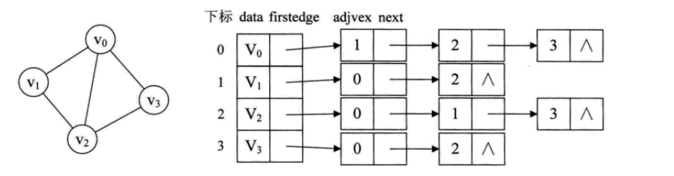
- 邻接表法
- 邻接矩阵法

图的元素
//edge
package basic_class_06;
public class Edge {
    public int weight;
    public Node from;
    public Node to;
    public Edge(int weight, Node from, Node to) {
        this.weight = weight;
        this.from = from;
        this.to = to;
    }
}
//Graph
package basic_class_06;
import java.util.HashMap;
import java.util.HashSet;
public class Graph {
    public HashMap<Integer,Node> nodes;
    public HashSet<Edge> edges;
    public Graph() {
        nodes = new HashMap<>();
        edges = new HashSet<>();
    }
}
//GraphGenerator
package basic_class_06;
public class GraphGenerator {
    public static Graph createGraph(Integer[][] matrix) {
        Graph graph = new Graph();
        for (int i = 0; i < matrix.length; i++) {
            Integer weight = matrix[i][0];
            Integer from = matrix[i][1];
            Integer to = matrix[i][2];
            if (!graph.nodes.containsKey(from)) {
                graph.nodes.put(from, new Node(from));
            }
            if (!graph.nodes.containsKey(to)) {
                graph.nodes.put(to, new Node(to));
            }
            Node fromNode = graph.nodes.get(from);
            Node toNode = graph.nodes.get(to);
            Edge newEdge = new Edge(weight, fromNode, toNode);
            fromNode.nexts.add(toNode);
            fromNode.out++;
            toNode.in++;
            fromNode.edges.add(newEdge);
            graph.edges.add(newEdge);
        }
        return graph;
    }
}
//node
package basic_class_06;
import java.util.ArrayList;
public class Node {
    public int value;
    public int in;
    public int out;
    public ArrayList<Node> nexts;
    public ArrayList<Edge> edges;
    public Node(int value) {
        this.value = value;
        in = 0;
        out = 0;
        nexts = new ArrayList<>();
        edges = new ArrayList<>();
    }
}
图的宽度优先遍历
- 利用队列实现
- 从源节点开始依次按照宽度进队列,然后弹出
- 每弹出一个点,把该节点所有没进过队列的邻接点放入队列
- 知道队列变空
广度优先遍历
- 利用栈实现
- 从源节点开始把节点按照深度放入栈
- 每弹出一个点,把该节点所有没进过栈的邻接点放入栈
- 知道栈变空
//宽度优先遍历
package basic_class_06;
import java.util.HashSet;
import java.util.LinkedList;
import java.util.Queue;
public class Code_01_BFS {
    public static void bfs(Node node) {
        if (node == null) {
            return;
        }
        Queue<Node> queue = new LinkedList<>();
        HashSet<Node> map = new HashSet<>();
        queue.add(node);
        map.add(node);
        while (!queue.isEmpty()) {
            Node cur = queue.poll();
            System.out.println(cur.value);
            for (Node next : cur.nexts) {
                if (!map.contains(next)) {
                    map.add(next);
                    queue.add(next);
                }
            }
        }
    }
}
//深度优先遍历
package basic_class_06;
import java.util.HashSet;
import java.util.Stack;
public class Code_02_DFS {
public static void dfs(Node node) {
if (node == null) {
return;
}
Stack<Node> stack = new Stack<>();
HashSet<Node> set = new HashSet<>();
stack.add(node);
set.add(node);
System.out.println(node.value);
while (!stack.isEmpty()) {
Node cur = stack.pop();
for (Node next : cur.nexts) {
if (!set.contains(next)) {
stack.push(cur);
stack.push(next);
set.add(next);
System.out.println(next.value);
break;
}
}
}
}
}拓扑排序算法
package basic_class_06;

import java.util.ArrayList;
import java.util.HashMap;
import java.util.LinkedList;
import java.util.List;
import java.util.Queue;

public class Code_03_TopologySort {

    // directed graph and no loop
    public static List<Node> sortedTopology(Graph graph) {
        HashMap<Node, Integer> inMap = new HashMap<>();
        Queue<Node> zeroInQueue = new LinkedList<>();
        for (Node node : graph.nodes.values()) {
            inMap.put(node, node.in);
            if (node.in == 0) {
                zeroInQueue.add(node);
            }
        }
        List<Node> result = new ArrayList<>();
        while (!zeroInQueue.isEmpty()) {
            Node cur = zeroInQueue.poll();
            result.add(cur);
            for (Node next : cur.nexts) {
                inMap.put(next, inMap.get(next) - 1);
                if (inMap.get(next) == 0) {
                    zeroInQueue.add(next);
                }
            }
        }
        return result;
    }
}
package basic_class_06;
import java.util.ArrayList;
import java.util.HashMap;
import java.util.LinkedList;
import java.util.List;
import java.util.Queue;
public class Code_03_TopologySort {
// directed graph and no loop
public static List<Node> sortedTopology(Graph graph) {
HashMap<Node, Integer> inMap = new HashMap<>();
Queue<Node> zeroInQueue = new LinkedList<>();
for (Node node : graph.nodes.values()) {
inMap.put(node, node.in);
if (node.in == 0) {
zeroInQueue.add(node);
}
}
List<Node> result = new ArrayList<>();
while (!zeroInQueue.isEmpty()) {
Node cur = zeroInQueue.poll();
result.add(cur);
for (Node next : cur.nexts) {
inMap.put(next, inMap.get(next) - 1);
if (inMap.get(next) == 0) {
zeroInQueue.add(next);
}
}
}
return result;
}
}Kruskal——求最小生成树

package basic_class_06;

import java.util.Collection;
import java.util.Comparator;
import java.util.HashMap;
import java.util.HashSet;
import java.util.PriorityQueue;
import java.util.Set;

//undirected graph only
public class Code_04_Kruskal {

    // Union-Find Set
    public static class UnionFind {
        private HashMap<Node, Node> fatherMap;
        private HashMap<Node, Integer> rankMap;

        public UnionFind() {
            fatherMap = new HashMap<Node, Node>();
            rankMap = new HashMap<Node, Integer>();
        }

        private Node findFather(Node n) {
            Node father = fatherMap.get(n);
            if (father != n) {
                father = findFather(father);
            }
            fatherMap.put(n, father);
            return father;
        }

        public void makeSets(Collection<Node> nodes) {
            fatherMap.clear();
            rankMap.clear();
            for (Node node : nodes) {
                fatherMap.put(node, node);
                rankMap.put(node, 1);
            }
        }

        public boolean isSameSet(Node a, Node b) {
            return findFather(a) == findFather(b);
        }

        public void union(Node a, Node b) {
            if (a == null || b == null) {
                return;
            }
            Node aFather = findFather(a);
            Node bFather = findFather(b);
            if (aFather != bFather) {
                int aFrank = rankMap.get(aFather);
                int bFrank = rankMap.get(bFather);
                if (aFrank <= bFrank) {
                    fatherMap.put(aFather, bFather);
                    rankMap.put(bFather, aFrank + bFrank);
                } else {
                    fatherMap.put(bFather, aFather);
                    rankMap.put(aFather, aFrank + bFrank);
                }
            }
        }
    }

    public static class EdgeComparator implements Comparator<Edge> {

        @Override
        public int compare(Edge o1, Edge o2) {
            return o1.weight - o2.weight;
        }

    }
//Kruskal
    public static Set<Edge> kruskalMST(Graph graph) {
        UnionFind unionFind = new UnionFind();
        unionFind.makeSets(graph.nodes.values());
        PriorityQueue<Edge> priorityQueue = new PriorityQueue<>(new EdgeComparator());
        for (Edge edge : graph.edges) {
            priorityQueue.add(edge);
        }
        Set<Edge> result = new HashSet<>();
        while (!priorityQueue.isEmpty()) {
            Edge edge = priorityQueue.poll();
            if (!unionFind.isSameSet(edge.from, edge.to)) {
                result.add(edge);
                unionFind.union(edge.from, edge.to);
            }
        }
        return result;
    }
}prim——无向图求最小生成树
| 图例 | 说明 | 不可选 | 可选 | 已选(Vnew) |
|---|---|---|---|---|
 |
此为原始的加权连通图。每条边一侧的数字代表其权值。 | - | - | - |
 |
顶点D被任意选为起始点。顶点A、B、E和F通过单条边与D相连。A是距离D最近的顶点,因此将A及对应边AD以高亮表示。 | C, G | A, B, E, F | D |
 |
下一个顶点为距离D或A最近的顶点。B距D为9,距A为7,E为15,F为6。因此,F距D或A最近,因此将顶点F与相应边DF以高亮表示。 | C, G | B, E, F | A, D |
 |
算法继续重复上面的步骤。距离A为7的顶点B被高亮表示。 | C | B, E, G | A, D, F |
 |
在当前情况下,可以在C、E与G间进行选择。C距B为8,E距B为7,G距F为11。E最近,因此将顶点E与相应边BE高亮表示。 | 无 | C, E, G | A, D, F, B |
 |
这里,可供选择的顶点只有C和G。C距E为5,G距E为9,故选取C,并与边EC一同高亮表示。 | 无 | C, G | A, D, F, B, E |
 |
顶点G是唯一剩下的顶点,它距F为11,距E为9,E最近,故高亮表示G及相应边EG。 | 无 | G | A, D, F, B, E, C |
 |
现在,所有顶点均已被选取,图中绿色部分即为连通图的最小生成树。在此例中,最小生成树的权值之和为39。 | 无 | 无 | A, D, F, B, E, C, G |
package basic_class_06;

import java.util.Comparator;
import java.util.HashSet;
import java.util.PriorityQueue;
import java.util.Set;

// undirected graph only
public class Code_05_Prim {

    public static class EdgeComparator implements Comparator<Edge> {

        @Override
        public int compare(Edge o1, Edge o2) {
            return o1.weight - o2.weight;
        }

    }

    public static Set<Edge> primMST(Graph graph) {
        PriorityQueue<Edge> priorityQueue = new PriorityQueue<>(
                new EdgeComparator());
        HashSet<Node> set = new HashSet<>();
        Set<Edge> result = new HashSet<>();
        for (Node node : graph.nodes.values()) {
            if (!set.contains(node)) {
                set.add(node);
                for (Edge edge : node.edges) {
                    priorityQueue.add(edge);
                }
                while (!priorityQueue.isEmpty()) {
                    Edge edge = priorityQueue.poll();
                    Node toNode = edge.to;
                    if (!set.contains(toNode)) {
                        set.add(toNode);
                        result.add(edge);
                        for (Edge nextEdge : toNode.edges) {
                            priorityQueue.add(nextEdge);
                        }
                    }
                }
            }
        }
        return result;
    }

}
Dijkstra
ps:不能有权值为负数的环
假设有下面这个图:

Dijkstra 算法将会寻找出图中节点 0 到所有其他节点的最短路径。
💡 提示: 在这个图中,我们假定两个节点之间的权重表示它们之间的距离。
我们将会得到节点 0 到节点 1、节点 0 到节点 2、节点 0 到 节点 3……(以此类推)的最短路径。
初始的距离列表如下:
- 源节点到它自身的距离为
0。示例中的源节点定为节点0,不过你也可以选择任意其它节点作为源节点。 - 源节点到其它节点的距离还没有确定,所以先标记为无穷大。

还有一个列表用来记录哪些节点未被访问(即尚未被包含在路径中):

💡 提示: 记住,当所有节点都被添加到路径中时,算法的计算过程就完成了。
我们选择了从节点 0 出发,可以直接将它标记为“已访问”,同样的,在未访问节点列表中把它划掉,并在图中给它加上红色的边框:


现在需要检查节点 0 到相邻节点的距离,两个相邻节点分别是节点 1 和节点 2(注意看红色的边):

💡 提示: 这并不是说立即把这两个相邻节点加入到最短路径中。在把一个节点加入到最短路径之前,需要确认是否已经寻找到了访问它的最短路径。现在只是在对可选方案做初步检查。
更新节点 0 到节点 1、节点 0 到节点 2 的距离为它们之间的边的权重,分别为 2 和 6:

更新了到相邻节点的距离之后:
- 根据已知的距离列表选择距离源节点最近的节点。
- 将它标记为“已访问”。
- 将它添加到路径中。
查看距离列表,发现节点 1 到源节点的距离是最短的(距离为 2),所以把它加入到路径中。
在图中,以红色边来表示:

在距离列表中用红色方块标记这个节点,表明它是“已访问”的、已经寻找到了访问这个节点的最短路径:

在未访问节点列表中将它划掉:

现在分析新的相邻节点,寻找访问它们的最短路径。只需要分析已经在最短路径(标记为红色边)中的节点的相邻节点。
节点 2 和节点 3 都是最短路径包含的节点的相邻节点,因为它们分别与节点 0 和节点 1 直接相连,如下图所示。下一步将要分析这两个节点。

之前已经计算过源节点到节点 2 的距离,并记录在了列表中,所以不用更新。这次只需要更新源节点到新的相邻节点(节点 3)的距离:

这个距离是 7,来看看为什么。
为了计算源节点到另一个节点(这里指节点 3)的距离,需要把访问该节点的最短路径的所有边权重相加:
- 对于节点
3: 将构成路径0 -> 1 -> 3的所有边权重相加,得到总距离为 7(0 -> 1距离为 2,1 -> 3距离为 5)。

现在得到了到相邻节点的距离,需要选择一个节点添加到路径中。我们必须选择一个已知到源节点距离最短的未访问节点。
从距离列表中可以看出,距离为 6 的节点 2 就是我们的选择:

在图中为它加上红色边框,并将路径上的边标记为红色:

在距离列表中用红色方块把它标记为“已访问”,在“未访问”节点列表中把它划掉:


重复前面的步骤,寻找源节点到新的相邻节点节点 3 的最短路径。
可以看到,有两种可选的路径:0 -> 1 -> 3 或 0 -> 2 -> 3。一起看看我们是如何确定最短路径的。

节点 3 在之前已经有了一个距离记录(距离为 7,参阅下表),这个距离是之前步骤中由路径 0 -> 1 -> 3 的两个边权重(分别为 5 和 2)相加得到的。
不过现在有了一个新的可选路径:0 -> 2 -> 3,它途经权重分别为 6 和 8 的两条边 0 -> 2 和 2 -> 3,总距离为 14。

显然,第一个路径的距离更短(7 vs. 14),所以选择第一个路径 0 -> 1 -> 3。只有在新的路径距离更短的情况下,才会更新距离列表。
因此,使用第一种方案 0 -> 1 -> 3,将节点添加到路径中。

把这个节点标记为“已访问”,在“未访问”节点列表中把它划掉:


重复前面的过程。
检查尚未访问的相邻节点:节点 4 和节点 5,因为它们是节点 3 的相邻节点。

更新它们到源节点的距离,尝试寻找更短的路径:
- 对于节点
4: 路径是0 -> 1 -> 3 -> 4,距离为 17。 - 对于节点
5: 路径是0 -> 1 -> 3 -> 5,距离为 22。
💡 提示: 注意我们只能从最短路径(红色边)上进行扩展,而不能途经未被包含在最短路径中的边(例如,不能构造经过边 2 -> 3 的路径)。

现在需要选择将哪个未访问节点标记为“已访问”,这里选择节点 4,因为在距离列表中它的距离最短。在图中做标记:

在距离列表中用红色方块将它标记为“已访问”:

在“未访问”节点列表中把它划掉:

再次重复前面的过程。检查相邻节点:节点 5 和节点 6。分析每一种从已访问节点到它们之间的可能路径方案。

对于节点 5:
- 第一种选择是路径
0 -> 1 -> 3 -> 5,到源节点的距离为 22(2 + 5 + 15),前面的步骤已经记录了这个距离。 - 第二种选择是路径
0 -> 1 -> 3 -> 4 -> 5,到源节点的距离为 23(2 + 5 + 10 + 6)。
显然,第一个路径距离更短,为节点 5 选择第一种方案。
对于节点 6:
- 可选的路径是
0 -> 1 -> 3 -> 4 -> 6,到源节点的距离为 19(2 + 5 + 10 + 2)。

把距离最短(当前已知)的节点 6 标记为“已访问”。

在“未访问”节点列表中把它划掉:

现在得到了如下路径(标记为红色):

现在只剩下一个节点 5 还没被访问了,看看我们要如何把它添加到路径中。
从已经添加到路径中的节点出发,有三种不同的路径可以访问节点 5:
- 第一种选择:
0 -> 1 -> 3 -> 5,总距离为 22(2 + 5 + 15)。 - 第二种选择:
0 -> 1 -> 3 -> 4 -> 5,总距离为 23(2 + 5 + 10 + 6)。 - 第三种选择:
0 -> 1 -> 3 -> 4 -> 6 -> 5,总距离为 25(2 + 5 + 10 + 2 + 6)。

选择总距离为 22 的最短路径:0 -> 1 -> 3 -> 5。

把这个节点标记为“已访问”,并在“未访问”节点列表中把它划掉:


瞧! 我们得到了从节点 0 到图中每个节点的最短路径。

图中,标记为红色的边表示最短路径:连接节点 0 和目标节点的红色边即为从源节点出发访问目标节点的最短路径。
例如,想要从节点 0 出发访问节点 6,连接它们的红色边就是最短路径,跟着走就行了。
package basic_class_06;
import java.util.HashMap;
import java.util.HashSet;
import java.util.Map.Entry;
// no negative weight
public class Code_06_Dijkstra {
    public static HashMap<Node, Integer> dijkstra1(Node head) {
        HashMap<Node, Integer> distanceMap = new HashMap<>();
        distanceMap.put(head, 0);
        HashSet<Node> selectedNodes = new HashSet<>();
        Node minNode = getMinDistanceAndUnselectedNode(distanceMap, selectedNodes);
        while (minNode != null) {
            int distance = distanceMap.get(minNode);
            for (Edge edge : minNode.edges) {
                Node toNode = edge.to;
                if (!distanceMap.containsKey(toNode)) {
                    distanceMap.put(toNode, distance + edge.weight);
                }
                distanceMap.put(edge.to, Math.min(distanceMap.get(toNode), distance + edge.weight));
            }
            selectedNodes.add(minNode);
            minNode = getMinDistanceAndUnselectedNode(distanceMap, selectedNodes);
        }
        return distanceMap;
    }
    public static Node getMinDistanceAndUnselectedNode(HashMap<Node, Integer> distanceMap,
            HashSet<Node> touchedNodes) {
        Node minNode = null;
        int minDistance = Integer.MAX_VALUE;
        for (Entry<Node, Integer> entry : distanceMap.entrySet()) {
            Node node = entry.getKey();
            int distance = entry.getValue();
            if (!touchedNodes.contains(node) && distance < minDistance) {
                minNode = node;
                minDistance = distance;
            }
        }
        return minNode;
    }
    public static class NodeRecord {
        public Node node;
        public int distance;

        public NodeRecord(Node node, int distance) {
            this.node = node;
            this.distance = distance;
        }
    }
    public static class NodeHeap {
        private Node[] nodes;
        private HashMap<Node, Integer> heapIndexMap;
        private HashMap<Node, Integer> distanceMap;
        private int size;

        public NodeHeap(int size) {
            nodes = new Node[size];
            heapIndexMap = new HashMap<>();
            distanceMap = new HashMap<>();
            this.size = 0;
        }
        public boolean isEmpty() {
            return size == 0;
        }

        public void addOrUpdateOrIgnore(Node node, int distance) {
            if (inHeap(node)) {
                distanceMap.put(node, Math.min(distanceMap.get(node), distance));
                insertHeapify(node, heapIndexMap.get(node));
            }
            if (!isEntered(node)) {
                nodes[size] = node;
                heapIndexMap.put(node, size);
                distanceMap.put(node, distance);
                insertHeapify(node, size++);
            }
        }
        public NodeRecord pop() {
            NodeRecord nodeRecord = new NodeRecord(nodes[0], distanceMap.get(nodes[0]));
            swap(0, size - 1);
            heapIndexMap.put(nodes[size - 1], -1);
            distanceMap.remove(nodes[size - 1]);
            nodes[size - 1] = null;
            heapify(0, --size);
            return nodeRecord;
        }

        private void insertHeapify(Node node, int index) {
            while (distanceMap.get(nodes[index]) < distanceMap.get(nodes[(index - 1) / 2])) {
                swap(index, (index - 1) / 2);
                index = (index - 1) / 2;
            }
        }
        private void heapify(int index, int size) {
            int left = index * 2 + 1;
            while (left < size) {
                int smallest = left + 1 < size && distanceMap.get(nodes[left + 1]) < distanceMap.get(nodes[left])
                        ? left + 1 : left;
                smallest = distanceMap.get(nodes[smallest]) < distanceMap.get(nodes[index]) ? smallest : index;
                if (smallest == index) {
                    break;
                }
                swap(smallest, index);
                index = smallest;
                left = index * 2 + 1;
            }
        }
        private boolean isEntered(Node node) {
            return heapIndexMap.containsKey(node);
        }

        private boolean inHeap(Node node) {
            return isEntered(node) && heapIndexMap.get(node) != -1;
        }

        private void swap(int index1, int index2) {
            heapIndexMap.put(nodes[index1], index2);
            heapIndexMap.put(nodes[index2], index1);
            Node tmp = nodes[index1];
            nodes[index1] = nodes[index2];
            nodes[index2] = tmp;
        }
    }
    public static HashMap<Node, Integer> dijkstra2(Node head, int size) {
        NodeHeap nodeHeap = new NodeHeap(size);
        nodeHeap.addOrUpdateOrIgnore(head, 0);
        HashMap<Node, Integer> result = new HashMap<>();
        while (!nodeHeap.isEmpty()) {
            NodeRecord record = nodeHeap.pop();
            Node cur = record.node;
            int distance = record.distance;
            for (Edge edge : cur.edges) {
                nodeHeap.addOrUpdateOrIgnore(edge.to, edge.weight + distance);
            }
            result.put(cur, distance);
        }
        return result;
    }
}
7.详解前缀树与贪心算法
前缀树(Trie树,字典树)
前缀树是N叉树的一种特殊形式。通常来说,一个前缀树是用来存储字符串的。前缀树的每一个节点代表一个字符串(前缀)。每一个节点会有多个子节点,通往不同子节点的路径上有着不同的字符。子节点代表的字符串是由节点本身的原始字符串,以及通往该子节点路径上所有的字符组成的。

值得注意的是,根节点表示空字符串。
前缀树的一个重要的特性是,节点所有的后代都与该节点相关的字符串有着共同的前缀。这就是前缀树名称的由来。
我们再来看这个例子。例如,以节点 "b" 为根的子树中的节点表示的字符串,都具有共同的前缀 "b"。反之亦然,具有公共前缀 "b" 的字符串,全部位于以 "b" 为根的子树中,并且具有不同前缀的字符串来自不同的分支。
前缀树有着广泛的应用,例如自动补全,拼写检查等等。我们将在后面的章节中介绍实际应用场景。
如何表示一个前缀树?
package class_07;
public class Code_01_TrieTree {
    public static class TrieNode {
        public int path;
        public int end;
        public TrieNode[] nexts;
        public TrieNode() {
            path = 0;
            end = 0;
            nexts = new TrieNode[26];
        }
    }
    public static class Trie {
        private TrieNode root;

        public Trie() {
            root = new TrieNode();
        }

        public void insert(String word) {
            if (word == null) {
                return;
            }
            char[] chs = word.toCharArray();
            TrieNode node = root;
            int index = 0;
            for (int i = 0; i < chs.length; i++) {
                index = chs[i] - 'a';
                if (node.nexts[index] == null) {
                    node.nexts[index] = new TrieNode();
                }
                node = node.nexts[index];
                node.path++;
            }
            node.end++;
        }
        public void delete(String word) {
            if (search(word) != 0) {
                char[] chs = word.toCharArray();
                TrieNode node = root;
                int index = 0;
                for (int i = 0; i < chs.length; i++) {
                    index = chs[i] - 'a';
                    if (--node.nexts[index].path == 0) {
                        node.nexts[index] = null;
                        return;
                    }
                    node = node.nexts[index];
                }
                node.end--;
            }
        }
        public int search(String word) {
            if (word == null) {
                return 0;
            }
            char[] chs = word.toCharArray();
            TrieNode node = root;
            int index = 0;
            for (int i = 0; i < chs.length; i++) {
                index = chs[i] - 'a';
                if (node.nexts[index] == null) {
                    return 0;
                }
                node = node.nexts[index];
            }
            return node.end;
        }
        public int prefixNumber(String pre) {
            if (pre == null) {
                return 0;
            }
            char[] chs = pre.toCharArray();
            TrieNode node = root;
            int index = 0;
            for (int i = 0; i < chs.length; i++) {
                index = chs[i] - 'a';
                if (node.nexts[index] == null) {
                    return 0;
                }
                node = node.nexts[index];
            }
            return node.path;
        }
    }
贪心算法
贪心算法(又称贪婪算法)是指,在对问题求解时,总是做出在当前看来是最好的选择。
也就是说,不从整体最优上加以考虑,他所做出的是在某种意义上的局部最优解。
贪心算法不是对所有问题都能得到整体最优解,关键是贪心策略的选择,选择的贪心策略必须具备无后效性,即某个状态以前的过程不会影响以后的状态,只与当前状态有关。
所做出的是某种意义上的局部最优
package basic_class_07;
import java.util.Arrays;
import java.util.Comparator;
public class Code_06_BestArrange {
    public static class Program {
        public int start;
        public int end;
        public Program(int start, int end) {
            this.start = start;
            this.end = end;
        }
    }
    public static class ProgramComparator implements Comparator<Program> {

        @Override
        public int compare(Program o1, Program o2) {
            return o1.end - o2.end;
        }
    }
    public static int bestArrange(Program[] programs, int start) {
        Arrays.sort(programs, new ProgramComparator());
        int result = 0;
        for (int i = 0; i < programs.length; i++) {
            if (start <= programs[i].start) {
                result++;
                start = programs[i].end;
            }
        }
        return result;
    }
    public static void main(String[] args) {
    }
}
你自己想出贪心策略,但只能感觉它对不对,理论证明放弃吧!重点在于想很多的贪心策略,用对数器去证明对不对。-
所谓贪心算法是指,在对问题求解时,总是做出在当前看来是最好的选择(最小,最大,最优等等)。也就是说,不从整体最优上加以考虑,它所做出的仅是在某种意义上的局部最优解。
-
贪心策略适用的前提是:局部最优策略能导致产生全局最优解。 【不要去理论证明你选择的贪心策略的正确性,因为太复杂,你最好直接看结果对不对就好】
-
贪心算法的基本思路:
1、建立数学模型来描述问题;
2、把求解的问题分成若干个子问题;
3、对每一子问题求解,得到子问题的局部最优解;4、把子问题的解局部最优解合成原来解问题的一个解
题目1:按最低字典序拼接字符串
题目:给定一个字符串类型的数组strs,找到一种拼接方式,使得把所有字符串拼起来之后形成的字符串具有最低的字典序。
字典序:对于两个字符串
长度不一样,将短的个补0(0是最小ASCII码值),补成长度一样;
先按首字符排序,如果首字符相同,再按第二个字符排序,以此类推。如aa,ab,ba,bb,bc就是一个字典序,从小到大。
【分析】贪心:你定一个指标,按这个指标来,对每个样本分出个优先,优先级大的先处理,优先级小的后处理。
本题的贪心策略就是你选择的比较策略
str1.str2 <= str2.str1,则 str1 放前面,否则 str2 放前面【根据两个字符串拼接的结果的大小来决定排序】,不能直接根据str1和str2的大小比较决定位置排放,比如:b和ba,最小的字典序应该是bab而不是bba。
package com.offer.foundation.class5;
import java.util.Arrays;
import java.util.Comparator;

public class Lowest {
    // 自定义比较器:给字符串按照自定义的规则排序
    public class MyComparator implements Comparator<String> {
        @Override
        public int compare(String a, String b) {
            return (a + b).compareTo(b + a);   // 哪个小哪个放前面
        }
    }
    public String getLowestString(String[] strs){
        if(strs == null || strs.length == 0){
            return "";
        }
        // 给字符串数组按照自己定义的规则排序
        // 对于制定的贪心策略,先直观分析下对不对,不要去试图证明,可以使用对数器证明
        Arrays.sort(strs, new MyComparator());
        String res = "";
        for (String str : strs) {
            res += str;
        }
        return res;
    }
    // 测试
    public static void main(String[] args) {
        Lowest lowest = new Lowest();
        String[] str = {"ba", "b","baa"};  // baabab
        System.out.println(lowest.getLowestString(str));
    }
}
题目2:切分金条总代价最小
题目:一块金条切成两半,是需要花费和长度数值一样的铜板的。比如:长度为20的金条,不管切成长度多大的两半,都要花费20个铜板。一群人想整分整块金条,怎么分最省铜板?
例如:给定数组{10, 20, 30},代表一共三个人,整块金条长度为 10+20+30=60. 金条要分成10, 20, 30三个部分。 如果, 先把长度60的金条分成10和50,花费60,再把长度50的金条分成20和30,花费50,一共花费110铜板。
但是如果先把长度60的金条分成30和30,花费60,再把长度30金条分成10和20,花费30 一共花费90铜板。
输入一个数组,返回分割的最小代价。
【分析】:贪心:每次合并代价最小的,设总代价为 cost = 0
1)把数组的元素放入优先队列(小根堆)中;
2)每次弹出最小的两个数【使其代价最小,因为贪心算法就是局部最优】,然后相加的结果为 c,总代价加上 c,并且将 c 放入堆中;
3)重复1)、2)步骤,直到堆中只剩有一个数结束。
【注意】: 优先队列是小根堆,你认为谁该在前面,就通过比较器把它的优先级设小【并不是实际数值小就在前面,也可能实际数值大在前面,看你比较器怎么弄了,返回负数:表示o1小于o2】
标准的霍夫曼编码问题:先选两个最小的合并,然后再往上合并(如下图所示)。合并是从下往上,切割的是从上往下:先将60切成30、30,再将其中一个30切成10、20,最后就将60切成:10、20、30

补充:堆结构的扩展与应用**【经常用于贪心】:**
堆:用于在一群数据中拿出最好的那个(根据自定义的比较器不同实现不同的堆,比较器就是贪心的标准),默认建的是小根堆(优先级小的放前面)。
package com.offer.foundation.class5;
import java.util.Comparator;
import java.util.PriorityQueue;
public class LowestCost {
    // 最小堆
    public class MyComparator implements Comparator<Integer>{
        @Override
        public int compare(Integer o1, Integer o2) {
            return o1 - o2;   // 谁小把谁放在前面: -表示o1小
        }
    }
    // 输入的是一个数组,数组中的元素则是最终的切割方式,现在要找出这种方式需要花费的最小代价
    public int lowestCost(int[] arr){
        // 优先级队列是小根堆,谁在前面,就把谁的优先级设置小点
        PriorityQueue<Integer> pq = new PriorityQueue<>(new MyComparator());
        for (int i : arr) {
            pq.add(i);
        }
        int costTotal = 0;   // 总的代价
        int costOne = 0;     // 两数合并的代价
        // 等于1的时候,说明堆里面只有一个元素了,即已经合并完成
        while(pq.size() > 1){
            costOne = pq.poll() + pq.poll();   // 合并堆里面最小的两个元素
            costTotal += costOne;              // 两小数合并的结果
            pq.add(costOne);                 // 将两小数合并的结果重新添加到堆里
        }
        return costTotal;
    }
    // 测试
    public static void main(String[] args) {
        LowestCost lc = new LowestCost();
        int[] arr = {10, 20, 30, 40};
        int res = lc.lowestCost(arr);
        System.out.println(res);      // 190 = 10 + 20 + 30 + 30 + 40 + 60
    }
}
以后遇到类似的问题,可以考虑下是否能够用霍夫曼编码的思想去解决。
题目3:最多做 K 个项目的最大利润
题目:costs[]:花费 ,costs[i] 表示 i 号项目的花费 profits[]:利润, profits[i] 表示 i 号项目在扣除花费之后还能挣到的钱(利润)。一次只能做一个项目,最多做 k 个项目,m 表示你初始的资金。(说明:你每做完一个项目,马上获得的收益,可以支持你去做下一个项目)求你最后获得的最大钱数。- 【分析】贪心:每次总是做能够做的项目中利润最大的。
- 准备一个小根堆和大根堆,小根堆放着全部的项目,按谁花费(成本)最低就在头部。
- 1、若小根堆不为空,项目也没做完 K 个,则每次先从小根堆解锁能够做的项目,放入大根堆(大根堆按照解锁的项目中谁的利润最大放在头部);
- 2、大根堆不为空,从大根堆弹出堆顶项目来做(即利润最大的项目,每次只弹出堆顶一个项目来做);
- 3、把 m 加上利润,初始资金增加,再重复1)、2)步骤。

注意:
- 解锁项目:只要项目成本在当前资金范围以内都可以被解锁,并不是一次只能解锁一个,然后按照利润的大小放进大根堆里,然后按照利润大的先做。所谓解锁项目其实就是资金肯定大于项目成本,该项目一定可以被做的,可以直观的感受下;
- 结束条件:可能做不到k个项目就会停了,因为可能存在成本比较高的项目,大根堆中可做的项目都做完了,总资金还是无法解锁成本比较大的项目,必须要停止了。
package com.offer.foundation.class5;
import java.util.Comparator;
import java.util.PriorityQueue;
/**
 * @author pengcheng
 * @date 2019/3/30 - 20:07
 * @content: 贪心算法:做多做k个项目的最大利润
 */
public class IPO {
    // 项目节点
    public class Node{
        private int profit;    // 项目利润
        private int cost;      // 项目成本

        public Node(int profit, int cost){
            this.profit = profit;
            this.cost = cost;
        }
    }
    /**
     * @param k :最多做k个项目
     * @param fund :总的资金
     * @param profits :每个项目的利润数组
     * @param cost :每个项目的成本数组
     * @return
     */
    public int findMaxCapital(int k, int fund, int[] profits, int[] cost){
        // 初始化每个项目节点信息
        Node[] nodes = new Node[profits.length];
        for (int i = 0; i < profits.length; i++) {
            nodes[i] = new Node(profits[i], cost[i]);
        }
        // 优先级队列是谁小谁放在前面,比较器决定谁小
        PriorityQueue<Node> minCostQ = new PriorityQueue<>(new MinCostComparator());       // 成本小顶堆
        PriorityQueue<Node> maxProfitQ = new PriorityQueue<>(new MaxProfitComparator());   // 利润大顶堆
        for (int i = 0; i < nodes.length; i++) {
            minCostQ.add(nodes[i]);   // 将所有的项目插入成本堆中
        }
        // 开始解锁项目,赚取利润
        for (int i = 0; i < k; i++) {
            // 解锁项目的前提条件:成本堆中还有项目未被解锁并且该项目的成本小于当前的总资金
            while(!minCostQ.isEmpty() && minCostQ.peek().cost <= fund){
                maxProfitQ.add(minCostQ.poll());   // 将当前成本最小的项目解锁
            }
            if(maxProfitQ.isEmpty()){
                // 如果maxProfitQ为空,则说明没有当前资金能够解锁的新项目了,之前解锁的项目也做完了,即无项目可做了
                return fund;   // 最后的总金额
            }
            fund += maxProfitQ.poll().profit;   // 做利润最大的项目
        }
        return fund;   // k个项目都做完了
    }
    // 成本小顶堆:成本最小的在堆顶
    public class MinCostComparator implements Comparator<Node>{
        @Override
        public int compare(Node o1, Node o2) {
            return o1.cost - o2.cost;
        }
    }
    // 利润大顶堆:利润最大的在堆顶
    public class MaxProfitComparator implements Comparator<Node>{
        @Override
        public int compare(Node o1, Node o2) {
            return o2.profit - o1.profit;
        }
    }
}
题目4:N皇后问题
n 皇后问题 研究的是如何将 n 个皇后放置在 n×n 的棋盘上,并且使皇后彼此之间不能相互攻击。
给你一个整数 n ,返回所有不同的 n 皇后问题 的解决方案。

package class23;

public class Code03_NQueens {

    public static int num1(int n) {
        if (n < 1) {
            return 0;
        }
        int[] record = new int[n];
        return process1(0, record, n);
    }

    // 当前来到i行,一共是0~N-1行
    // 在i行上放皇后,所有列都尝试
    // 必须要保证跟之前所有的皇后不打架
    // int[] record record[x] = y 之前的第x行的皇后,放在了y列上
    // 返回:不关心i以上发生了什么,i.... 后续有多少合法的方法数
    public static int process1(int i, int[] record, int n) {
        if (i == n) {
            return 1;
        }
        int res = 0;
        // i行的皇后,放哪一列呢?j列,
        for (int j = 0; j < n; j++) {
            if (isValid(record, i, j)) {
                record[i] = j;
                res += process1(i + 1, record, n);
            }
        }
        return res;
    }

    public static boolean isValid(int[] record, int i, int j) {
        // 0..i-1
        for (int k = 0; k < i; k++) {
            if (j == record[k] || Math.abs(record[k] - j) == Math.abs(i - k)) {
                return false;
            }
        }
        return true;
    }
常数优化:利用位运算加速
// 请不要超过32皇后问题
public static int num2(int n) {
    if (n < 1 || n > 32) {
        return 0;
    }
    // 如果你是13皇后问题,limit 最右13个1,其他都是0
    int limit = n == 32 ? -1 : (1 << n) - 1;
    return process2(limit, 0, 0, 0);
}

// 7皇后问题
// limit : 0....0 1 1 1 1 1 1 1
// 之前皇后的列影响:colLim
// 之前皇后的左下对角线影响:leftDiaLim
// 之前皇后的右下对角线影响:rightDiaLim
public static int process2(int limit, int colLim, int leftDiaLim, int rightDiaLim) {
    if (colLim == limit) {
        return 1;
    }
    // pos中所有是1的位置,是你可以去尝试皇后的位置
    int pos = limit & (~(colLim | leftDiaLim | rightDiaLim));
    int mostRightOne = 0;
    int res = 0;
    while (pos != 0) {
        mostRightOne = pos & (~pos + 1);
        pos = pos - mostRightOne;
        res += process2(limit,
                        colLim | mostRightOne,
                        (leftDiaLim | mostRightOne) << 1,
                        (rightDiaLim | mostRightOne) >>> 1);
    }
    return res;
}